How to create a Gantt chart in Excel?

When asked to name the three most important components of Microsoft Excel, which ones would you name? Most likely, sheets on which data is entered, formulas that are used to perform calculations, and charts, with the help of which data of various kinds can be represented graphically.

I am sure that every Excel user knows what a chart is and how to create one. However, there is a type of graph that is shrouded in obscurity for many - Gantt chart... This quick guide will explain the main features of a Gantt chart, tell you how to make a basic Gantt chart in Excel, tell you where to download advanced Gantt chart templates and how to use the online service "Project Management" to create Gantt charts.

What is a Gantt chart?

Gantt chart named after Henry Gantt, an American engineer and management consultant who came up with such a chart in 1910. A Gantt chart in Excel presents projects or tasks as a cascade of horizontal bar charts. The Gantt chart shows the structure of the project decomposed into parts (start and end dates, various relationships between tasks within the project) and thus helps to control the execution of tasks in time and according to the planned milestones.

How to create a Gantt chart in Excel 2010, 2007 and 2013

Unfortunately, Microsoft Excel does not offer a built-in Gantt chart template. However, you can quickly create one yourself using the functionality of a bar chart and a little formatting.

Follow these steps carefully and it will take less than 3 minutes to create a simple Gantt chart. In our examples, we create a Gantt chart in Excel 2010, but the same can be done in Excel 2007 and 2013.

Step 1. Create a project table

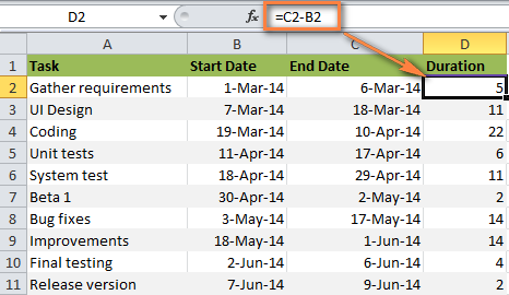
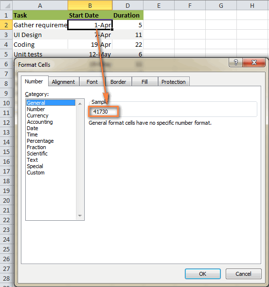
First of all, we will enter the project data into an Excel sheet. Write each task on a separate line and build a structural plan for the project by specifying start date(Start date), endings(End date) and duration(Duration), which is the number of days it takes to complete the task.

Advice: Only columns are required to create a Gantt chart Start date and Duration... However, if you also create a column End date, then you can calculate the duration of the task using a simple formula, as you can see in the figure below:

Step 2. Build a regular Excel bar chart based on the "Start date" column data

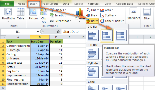
Start building a Gantt chart in Excel by creating a simple Stacked bar chart:

• Highlight a range Start dates along with the column heading, in our example it is B1: B11... You need to select only the cells with data, not the entire column of the sheet.
• In the tab Insert(Insert) under Charts, click Insert bar chart(Bar).
• In the menu that opens in the group Ruled(2-D Bar) click Stacked ruled(Stacked Bar).

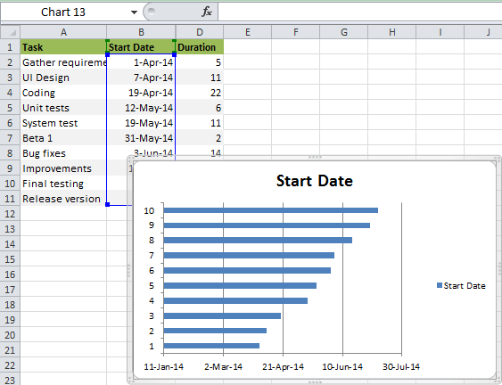
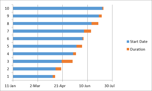
As a result, the following diagram should appear on the sheet:

Comment: Some other instructions for creating Gantt charts suggest that you first create an empty bar chart and then fill it with data, as we will do in the next step. But I think the method shown is better because Microsoft Excel will automatically add one row of data and thus save us some time.

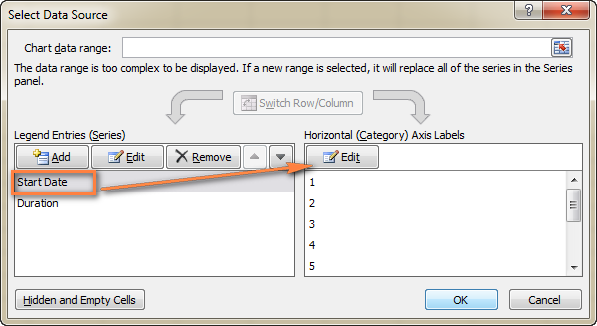
Step 3. Add duration data to the chart

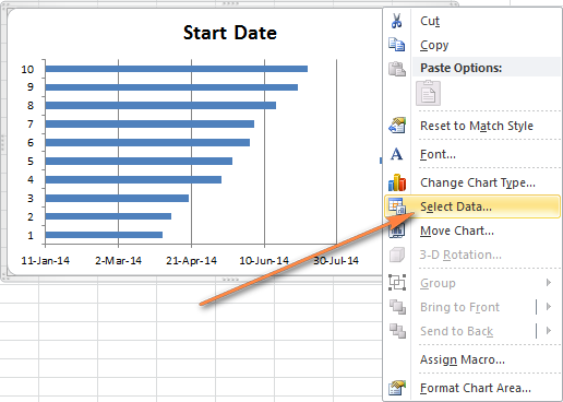
The diagram should look something like this:

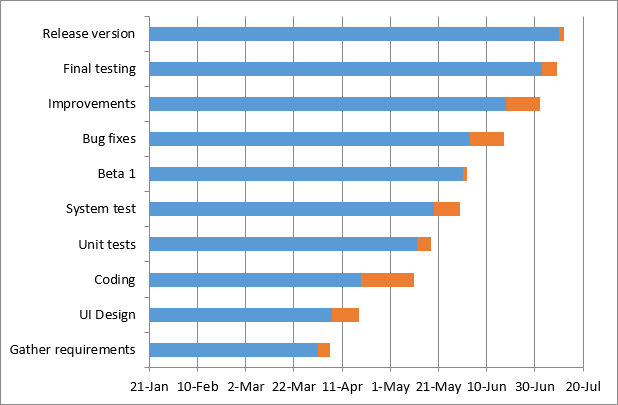
Step 4. Add task descriptions to the Gantt chart

Now you need to show a list of tasks on the left side of the diagram instead of numbers.

At this point, the Gantt chart should have task descriptions on the left side and look something like this:

Step 5: Turning a Bar Chart into a Gantt Chart

At this point, our chart is still a stacked bar chart. To make it look like a Gantt chart, you need to properly design it. Our task is to remove the blue lines so that only the orange parts of the graphs, which represent the project tasks, remain visible. Technically, we will not remove the blue lines, but simply make them transparent, which means invisible.

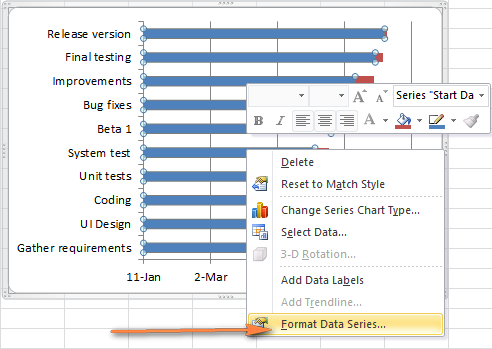
Comment: Do not close this dialog, you will need it again in the next step.

The chart becomes like a regular Gantt chart, right? For example, my Gantt chart now looks like this:

Step 6. Customize the design of the Gantt chart in Excel

The Gantt chart is already taking shape, but you can add a few more finishing touches to make it really stylish.

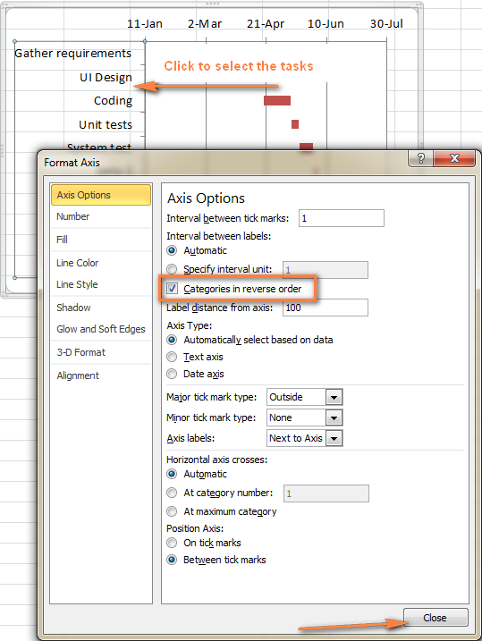
1. Remove the white space on the left side of the Gantt chart

When building a Gantt chart, at the beginning of the chart, we inserted blue bars showing the start date. Now the void that remained in their place can be removed and the task strips can be moved to the left, closer to the vertical axis.

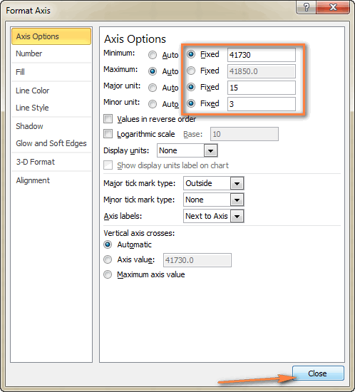
2. Adjust the number of dates on the axis of the Gantt chart

Here, in the dialog box Axis format(Format Axis) opened in the previous step, change the parameters Major divisions(Major unit) and Intermediate divisions(Minor unit) on Number(Fixed) and enter the desired axis spacing values. Usually, the shorter the time frame of tasks in the project, the smaller the step of divisions is needed on the time axis. For example, if you want to show every second date, then enter 2 for parameter Major divisions(Major unit). What settings I made - you can see in the picture below:

Advice: Play around with the parameter settings until you get the desired result. Don't be afraid to do something wrong, you can always return to the default settings by setting the parameters to Automatically(Auto) in Excel 2010 and 2007, or by clicking Reset(Reset) in Excel 2013.

3. Remove excess empty space between stripes

Arrange task bars on the chart more compactly, and the Gantt chart will look even better.

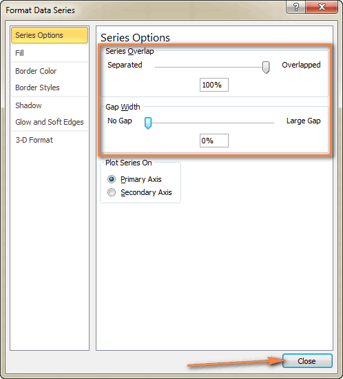
• Select the orange bars of the graphs by clicking on one of them with the left mouse button, then right-clicking on it and in the menu that appears, click Data series format(Format Data Series).
• In the dialog box Data series format(Format Data Series) set Overlapping rows(Series Overlap) is set to 100% (the slider is moved all the way to the right), and for the parameter Side clearance(Gap Width) value 0% or almost 0% (slider all the way or almost all the way to the left).

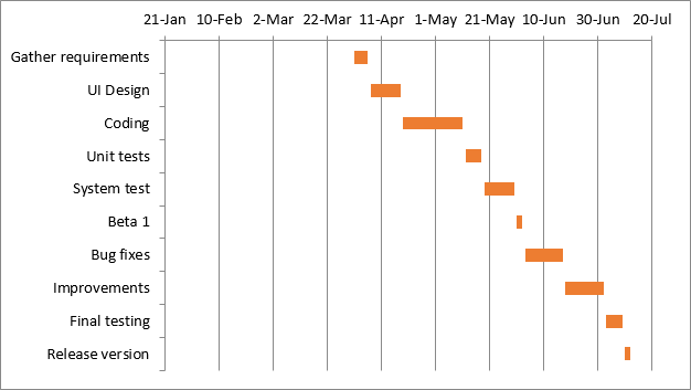
And here is the result of our efforts - a simple, but quite neat Gantt chart in Excel:

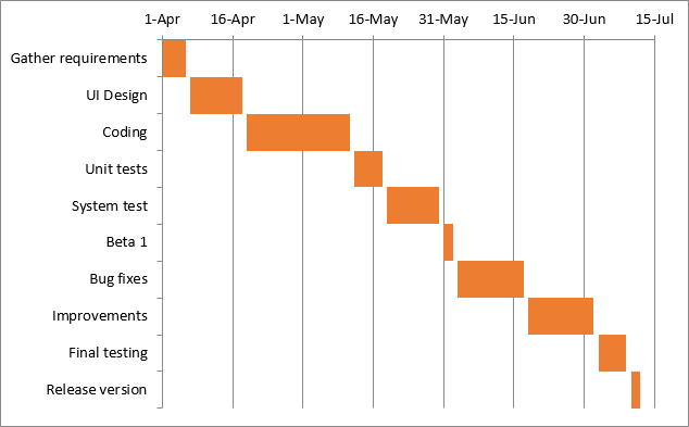
Remember that an Excel chart created in this way is very close to a real Gantt chart, while still retaining all the convenience of Excel charts:

• Gantt chart in Excel will resize when tasks are added or removed.
• Change the Start date or Duration of the task, and the graph will immediately automatically reflect the changes made.
• A Gantt chart created in Excel can be saved as a picture or converted to HTML format and published on the Internet.

Gantt chart templates in Excel

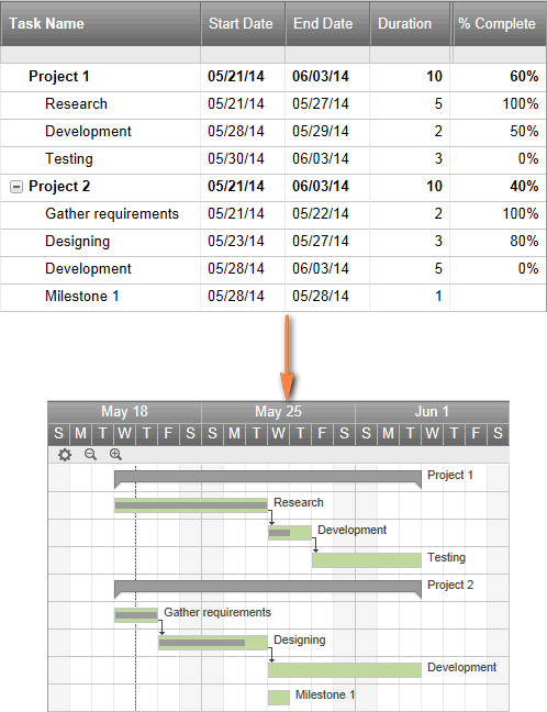
As you can see, building a simple Gantt chart in Excel is not difficult at all. But what if you need a more complex Gantt chart, in which the fill of the task depends on the percentage of its completion, and the control points of the project are indicated by vertical lines? Of course, if you are one of those rare and mysterious creatures that we respectfully call the Excel Guru, then you can try to make such a diagram yourself.

However, it will be faster and easier to use ready-made Gantt chart templates in Excel. Below is a quick overview of several project management Gantt chart templates for different versions of Microsoft Excel.

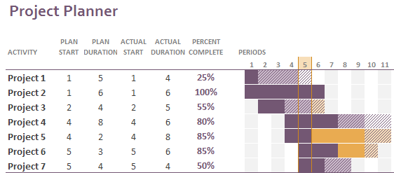
Gantt Chart Template for Excel 2013 from Microsoft

This Gantt chart template for Excel is called Project planner(Gantt Project Planner). It is designed to track the progress of a project by various metrics such as Planned start(Plan Start) and Actual start(Actual Start), Planned duration(Plan Duration) and Actual duration(Actual Duration) as well Percentage of completion(Percent Complete).

In Excel 2013, this template is available on the tab File(File) in the window Create(New). If there is no template in this section, you can download it from the Microsoft website. No additional knowledge is required to use this template - click on it and get started.

Online Gantt Chart Template

Smartsheet.com offers an interactive online Gantt chart builder. This Gantt chart template is as simple and ready to use as the previous one. The service offers a 30-day free trial, so sign up with your Google account and start creating your first Gantt chart right away.

The process is very simple: in the table on the left, enter the details of your project, and as the table fills out, a Gantt chart is created on the right.

Gantt Chart Templates for Excel, Google Sheets and OpenOffice Calc

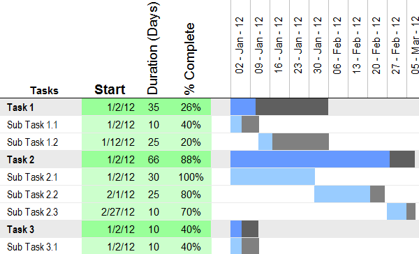
At vertex42.com you can find free Gantt chart templates for Excel 2003, 2007, 2010 and 2013 that will also work with OpenOffice Calc and Google Sheets. You can work with these templates in the same way as with any regular Excel spreadsheet. Just enter the start date and duration for each task and include the% completed in the column % Complete... To change the date range shown in the Gantt plot area, move the slider on the scroll bar.