Building the IDEF0 model

At the initial stages of creating an IP, it is necessary to understand how the organization that is going to be automated works. The manager knows the job well in general, but is not able to delve into the details of the work of each ordinary employee. An ordinary employee knows well what is happening in his workplace, but may not know how colleagues work. Therefore, to describe the work of an enterprise, it is necessary to build a model that will be adequate to the subject area and contain the knowledge of all participants in the organization's business processes.

The most convenient language for modeling business processes is IDEF0, where the system is represented as a set of interacting activities or functions. This purely functional orientation is fundamental - the functions of the system are analyzed independently of the objects with which they operate. This allows you to more clearly model the logic and interaction of the organization's processes.

The process of modeling a system in IDEF0 begins with the creation of a context diagram - a diagram of the most abstract level of describing the system as a whole, containing the definition of the subject of modeling, the goal and point of view on the model.

The subject is understood as the system itself, while it is necessary to establish exactly what is included in the system and what lies outside of it, in other words, to determine what will be further considered as components of the system and what as an external influence. The definition of the subject of the system will be significantly influenced by the position from which the system is viewed, and the purpose of modeling is the questions that the constructed model should answer. In other words, you first need to define the modeling area. The description of the area of ​​both the system as a whole and its components is the basis for building the model. Although it is assumed that the area can be adjusted during the simulation, it should be mainly formulated initially, since it is the area that determines the direction of the modeling. When formulating an area, there are two components to consider - breadth and depth. Latitude implies defining the boundaries of the model - what will be considered inside the system and what will be outside. Depth determines at what level of detail the model is complete. When determining the depth of the system, it is necessary to remember about time constraints - the complexity of building a model grows exponentially with an increase in the depth of decomposition. After defining the boundaries of the model, it is assumed that new objects should not be introduced into the modeled system.

Purpose of modeling

The goal of the simulation is determined by answering the following questions:

• Why should this process be modeled?
• What should the model show?
• What can a client get?

Viewpoint.

The point of view refers to the perspective from which the system was observed when building the model. Although the views of different people are taken into account when building the model, they should all adhere to the same point of view on the model. The point of view should be consistent with the purpose and boundaries of the simulation As a rule, the point of view of the person responsible for the simulated work as a whole is chosen.

The IDEF0 model assumes the presence of a clearly formulated goal, a single subject of modeling and one point of view. To enter the area, goal and point of view in the IDEF0 model in BPwin, select the Model / Model Properties menu item, which calls the Model Properties dialog (Fig. A2.3). On the Purpose tab, enter the goal and point of view, and on the Definition tab, the model definition and scope description.

Rice. A2.3. Dialogue for setting model properties

In the Status tab of the same dialog, you can describe the status of the model (draft, working, final, etc.), the time of creation and last editing (tracked later automatically by the system date). The Source tab describes the sources of information for building the model (for example, "Interviewing Domain Experts and Analyzing Documentation"). The General tab is used to enter the name of the project and the model, the name and initials of the author, and the time frame of the model - AS-IS and TO-BE.

AS-IS and TO-BE models. Usually, a model of the existing work organization is built first - AS-IS (as is). The analysis of the functional model allows you to understand where the weakest points are, what will be the advantages of new business processes and how deeply the existing structure of the business organization will undergo changes. The granularity of business processes makes it possible to identify the shortcomings of an organization even where functionality seems obvious at first glance. The shortcomings found in the AS-IS model can be corrected by creating a TO-BE model (as it will be) - a model of a new organization of business processes.

The IS design technology implies first the creation of an AS-IS model, its analysis and improvement of business processes, that is, the creation of a TO-BE model, and only on the basis of the TO-BE model a data model, a prototype and then the final version of the IS is built.

Sometimes the current AS-IS and future TO-BE models differ greatly, so that the transition from the initial to the final state becomes unclear. In this case, a third model is needed, which describes the process of transition from the initial to the final state of the system, since such a transition is also a business process.

The result of the description of the model can be obtained in the Model Report. The dialog for setting up a model report is called from the Tools / Reports / Model Report menu item.

In the settings dialog, select the required fields, and the order of information output to the report is automatically displayed (Fig. A2.4).

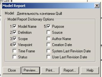
Rice. A2.4. Dialog box for generating a report on the model

In fig. A2.5 presents a report generated by the above fields.

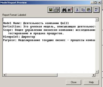
Rice. A2.5. Report preview

The basis of the IDEF0 methodology is a graphical language for describing business processes. A model in IDEF0 notation is a collection of hierarchically ordered and interconnected diagrams. Each diagram is a unit of system description and is located on a separate sheet.

The model can contain four types of charts:

• context diagram (each model can have only one context diagram);
• decomposition diagrams;
• node tree diagrams;
• exposure-only diagrams (FEO).

The context diagram is the top of the diagram tree structure and represents the most general description of the system and its interaction with the external environment. After describing the system as a whole, it is divided into large fragments. This process is called functional decomposition, and the diagrams that describe each fragment and the interaction of the fragments are called decomposition diagrams. After decomposition of the context diagram, each large fragment of the system is decomposed into smaller ones, and so on, until the required level of description is reached. After each decomposition session, examination sessions are held - subject area experts indicate the correspondence of real business processes to the created diagrams. The found inconsistencies are corrected, and only after passing the examination without comments, you can proceed to the next decomposition session. This is how the model matches the real business processes at any and every level of the model. The syntax for describing the system as a whole and each of its fragments is the same throughout the model.

The node tree diagram shows the hierarchical relationship of activities, but not the relationship between activities. There can be arbitrarily many node tree diagrams in the model, since the tree can be built to an arbitrary depth and not necessarily from the root.

exposure diagrams (FEO) are constructed to illustrate individual portions of a model, to illustrate an alternative point of view, or for special purposes.

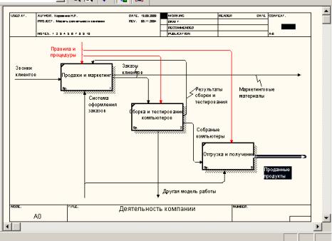
Work (Activity) denote named processes, functions, or tasks that occur over time and have recognizable results. The works are depicted as rectangles. All work must be named and defined. The name of the job must be expressed by a verbal noun denoting an action (for example, "Company activity", "Taking an order", etc.). The work "Company Activities" may have, for example, the following definition: "This is a training model describing the activities of a company." When creating a new model (File / New menu), a context diagram is automatically created with a single work depicting the system as a whole (Fig. A2.6).

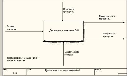
Rice. A2.6. Example of a context diagram

To enter a name for a job, right-click on the job, select Name Editor from the menu, and enter the name of the job in the dialog that appears. The Activity Properties dialog is used to describe other work properties (Fig. A2.7).

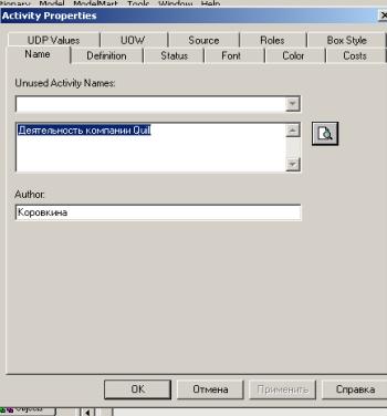
Rice. P2.P2. Job Properties Set Editor

Decomposition diagrams contain related activities, that is, child activities that have a common parent activity. To create a decomposition diagram, click on the button on the toolbar.

The Activity Box Count dialog appears (Fig. A2.8), in which you should specify the notation of the new diagram and the number of works on it. Let's dwell on the IDEF0 notation for now and click on OK. A decomposition diagram appears (Fig. A2.9). The allowed interval for the number of jobs is 2-8. It makes no sense to decompose a job into one job: diagrams with more than eight jobs turn out to be oversaturated and poorly readable. To provide clarity and better understanding of the simulated processes, it is recommended to use from three to six blocks in one diagram.

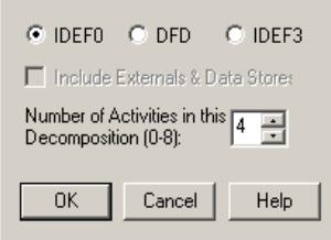
Rice. A2.8. Activity Box Count Dialogue

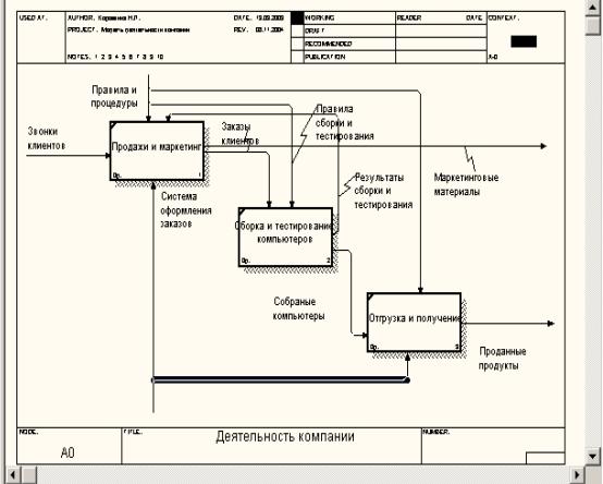
Rice. A2.9. Decomposition diagram example

If it turns out that the number of jobs is not enough, then the job can be added to the diagram by first clicking on the button on the tool palette, and then on the free space on the diagram.

Work in decomposition diagrams is usually arranged diagonally from the top left corner to the bottom right corner.

This order is called the dominance order. According to this principle of location, the most important work or the work performed first in time is placed in the upper left corner. Further down to the right are less important or later work. This arrangement makes the diagrams easier to read, and also provides a basis for the concept of work relationships (see below).

Each of the activities in the decomposition diagram can be decomposed in turn. In the breakdown diagram, jobs are numbered automatically from left to right. The job number is shown in the lower right corner. In the upper left corner, there is a small diagonal line, which indicates that this work has not been decomposed. So, in fig. A2.9 all jobs have not yet been decomposed.

Arrows describe the interaction of jobs and represent some kind of information expressed in nouns. (For example, "Customer Calls", "Rules and Procedures", "Accounting System".)

IDEF0 distinguishes between five types of arrows:

entrance(Input) - material or information that is used or transformed by work to obtain a result (output). It is assumed that the work may not have any entry arrows. Each type of arrow goes to or from a specific side of the work rectangle. The entry arrow is drawn as entering the left side of the work. When describing technological processes (for this, IDEF0 was invented), there are no problems with defining inputs. Indeed, the "Customer Calls" in fig. P2.6 is something that is processed in the "Company Activity" process to obtain a result. When modeling IS, when the arrows are not physical objects, but data, not everything is so obvious. For example, when "Admitting a patient", the patient record can be both at the entrance and at the exit, meanwhile the quality of this data changes. In other words, in our example, in order to justify its purpose, the entry and exit arrows must be precisely defined in order to indicate that the data has actually been processed (for example, the exit is "Completed Patient Record"). It is often difficult to determine if the data is input or control. In this case, information about whether the data is being processed / changed in operation or not can serve as a hint. If they change, then, most likely, this is an input, if not, it is a control.

Control(Control) - the rules, strategies, procedures or standards that govern the work. Each job must have at least one control arrow. The control arrow is drawn as entering the top face of the work. In fig. A2.6 arrow "Rules and procedures" - management for the work "Company activities". Management affects work, but is not transformed by work. If the goal of the work is to change a procedure or strategy, then such a procedure or strategy will be the input for the work. In case of uncertainty in the status of the arrow (control or input), it is recommended to draw the control arrow.

Exit(Output) - material or information that is produced by the work. Each job must have at least one exit arrow. Working without results is meaningless and should not be modeled. The exit arrow is drawn as coming from the right edge of the work. In fig. A2.6 arrows "Marketing materials" and "Products sold" are the output for the work "Company activities".

Mechanism(Mechanism) - resources that perform work, for example, enterprise personnel, machines, devices, etc. The arrow of the mechanism is drawn as part of the lower edge of the work. In fig. A2.6 arrow "Accounting system" is a mechanism for the operation of "Company activities". At the analyst's discretion, the mechanism arrows may not appear in the model.

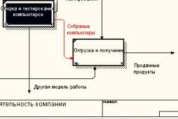
Call(Call) - a special arrow pointing to a different model of work. The call arrow is drawn as coming from the bottom edge of the work. In fig. A2.10 arrow "Another model of work" is a call for work "Manufacturing of a product". The call arrow is used to indicate that some work is being done outside the simulated system. In BPwin, call arrows are used in the model merge and split engine.

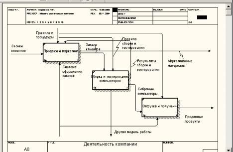
Rice. A2.10. Call arrow that appears when splitting a model

Boundary arrows. The arrows on the context diagram are used to describe the interaction of the system with the outside world. They can start at the border of the diagram and end at the work, or vice versa. These arrows are called boundary arrows.

To enter the boundary arrow of the entrance, you should:

Arrows for control, entry, mechanism and exit are depicted in the same way. The names of the newly added arrows (Fig. A2.11) are automatically entered into the Arrow Dictionary.

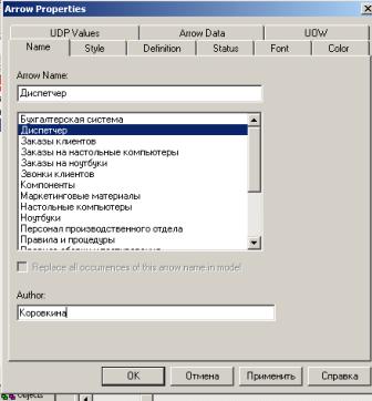
Rice. A2.11. IDEF0 Arrow Properties Dialogue

ICOM codes... The decomposition diagram is intended for detailing the work. Unlike models that display the structure of an organization, working in a top-level diagram in IDEF0 is not a control for subordinate activities. Low-level jobs are the same as high-level jobs, but in more detail. As a consequence, the boundaries of the top-level work are the same as the boundaries of the decomposition diagram. ICOM (acronym for Input, Control, Output and Mechanism) are codes designed to identify boundary arrows. The ICOM code contains a prefix corresponding to the type of arrow (I, C, O or M) and a sequence number.

BPwin fills in ICOM codes automatically. To display ICOM codes, enable the ICOM codes option on the Display tab of the Model Properties dialog (Model / Model Properties menu) (Fig. A2.12).

Vocabulary shooter edited with the help of a special editor Arrow Dictionary Editor, in which the arrow is defined and a comment related to it is added (Fig. A2.13). The arrow dictionary solves a very important problem. Diagrams are created by the analyst in order to conduct an examination session, that is, to discuss the diagram with a subject matter specialist. In any subject area, professional jargon is formed, and very often jargon expressions have a fuzzy meaning and are perceived by different specialists in different ways. At the same time, the analyst - the author of the diagrams should use those expressions that are most understandable to the experts. Since formal definitions are often difficult to understand, the analyst is forced to use professional jargon, and in order to avoid ambiguous interpretations, each concept can be given an extended and, if necessary, formal definition in the dictionary of arrows.

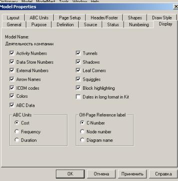
Rice. A2.12. Enabling ICOM codes option on the Display tab

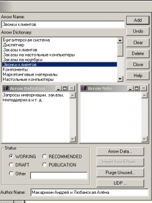
Rice. A2.13. Editing the arrow dictionary

The contents of the arrow dictionary can be printed as a report (menu Tools / Report / Arrow Report ...) and get an explanatory dictionary of the domain terms used in the model.

Unbound boundary arrows (unconnected border arrow)... When a job is decomposed, the arrows entering and leaving it (except for the call arrow) automatically appear on the decomposition diagram (arrow migration), but they do not touch the jobs. These arrows are called unbound arrows and are treated as a syntax error by BPwin.

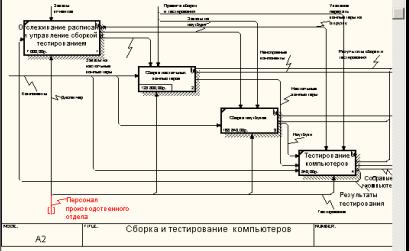
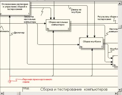
In fig. A2.14 shows a fragment of a decomposition diagram with unconnected arrows, generated by BPwin during work decomposition "Building Desktop Computers"(see Fig.A2.9). To link the arrows of the input, control or mechanism, you need to go to the edit mode of the arrows, click on the arrowhead and then on the corresponding segment of work. To link the exit arrow, go to the arrow edit mode, click on the work exit segment and then on the arrow.

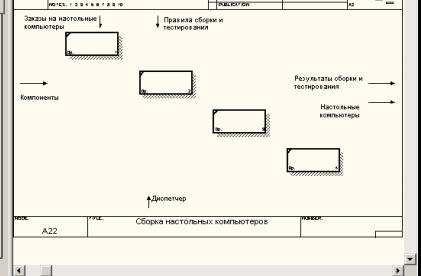
Rice. A2.14. An example of unbound arrows

Internal arrows. Internal arrows are used to connect the work to each other, that is, arrows that do not touch the border of the diagram, start at one and end at another work.

To draw the inner arrow, in the arrow drawing mode, click on a segment (for example, an exit) of one job and then on a segment (for example, an entrance) of another. IDEF0 distinguishes between five types of work relationships.

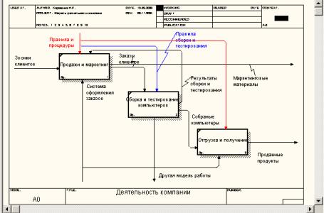
Input communication(output-input), when the arrow of the output of the higher-level work (hereinafter simply the output) is directed to the input of the lower-level work (for example, in Fig. A2.15 the arrow "Assembled Computers" connects works and "Shipping and receiving").

Rice. A2.15. Input communication

Management communication(output-control) when the output of a higher-level job is routed to the control of a lower-level job. The management link shows the dominance of the superior work. The data or output objects of a higher-level job do not change in the lower-level job. In fig. P2.16 arrow "Customer orders" connects works "Sales and Marketing" and "Assembling and testing computers".

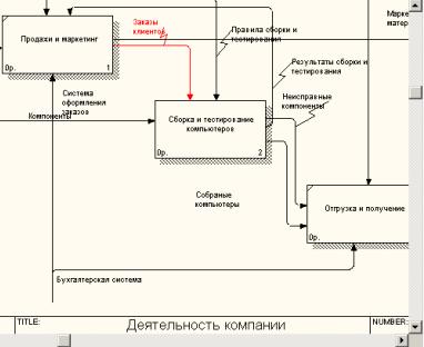
Rice. A2.16. Management communication

Input Feedback(output-input feedback) when the output of a lower-level job is routed to the input of a higher-level job. This relationship is usually used to describe loops. In fig. A2.17 arrow "Test results" connects works "Testing computers" and Schedule Tracking and Build and Test Management.

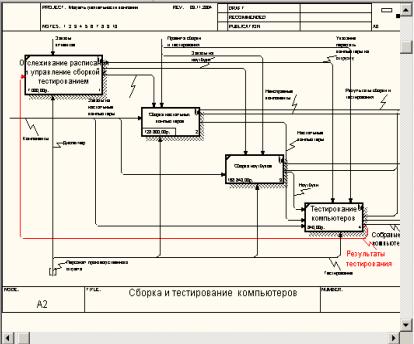
Rice. P2.1P2. Input Feedback

Management feedback(output-control feedback), when the output of the lower-level work is directed to the control of the higher-level one (arrow "Results of assembly and testing", Fig. A2.18). Management feedback is often indicative of the effectiveness of the business process. In fig. A2.18 sales volume can be increased by directly regulating the processes of assembling and testing computers (output) of the "Assembling and testing computers" work.

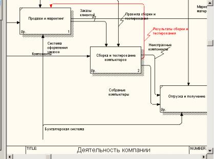
Rice. A2.18. Management feedback

Output-mechanism communication(output-mechanism), when the output of one work is directed to the mechanism of another. This relationship is used less often than others and shows that one job prepares the resources needed to carry out another job (Fig. A2.19).

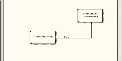
Rice. A2.19. Output-mechanism communication

Explicit arrows. An explicit arrow has a single job as a source and a single job as a destination.

Forking and merging arrows. The same data or objects generated by one job can be used in several other jobs at once. On the other hand, arrows generated in different works can represent the same or homogeneous data or objects that are later used or processed in one place. To simulate these situations, IDEF0 uses branching and merging arrows. To branch the arrow, in the arrow editing mode, click on the arrow fragment and on the corresponding segment of the work. To merge two exit arrows, in the arrow edit mode, first click on the segment of the work exit, and then on the corresponding fragment of the arrow.

The meaning of branching and merging arrows is conveyed by the naming of each branch of the arrows. There are certain rules for naming such arrows. Let's consider them on the example of branching arrows. If the arrow is named before the fork, and after the fork none of the branches is named, then it is assumed that each branch models the same data or objects as the branch before the fork (Fig. A2.20).

Rice. A2.20.

If the arrow is named before the branching, and after the branching any of the branches is also named, then it is implied that these branches correspond to the naming. If at the same time any branch remains unnamed after branching, then it is assumed that it models the same data or objects as the branch before branching (Fig. A2.21).

Rice. A2.21. Example of naming a branching arrow

The situation is unacceptable when the arrow is not named before the branch, and after the branch is not named any of the branches. BPwin defines this arrow as a syntax error.

The naming rules for merging arrows are completely similar - an error will be considered an arrow that is not named after the merge, and before the merge any of its branches were not named. To name a separate branch of branching and merging arrows, select only one branch on the diagram, then call the name editor and assign a name to the arrow. This name will only match the selected branch.

Tunneling arrows... Newly introduced boundary arrows on the lower-level decomposition diagram are shown in square brackets and do not automatically appear on the upper-level diagram (Fig. A2.22).

Rice. A2.22. Unresolved arrow

To "drag" them up, right-click on the square brackets of the boundary arrow and select the Arrow Tunnel command from the context menu (Fig. A2.23).

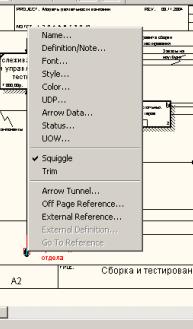
Rice. A2.23. Selecting a command from the context menu

The Border Arrow Editor dialog appears (Fig. A2.24).

If you click on the Resolve Border Arrow button, the arrow will migrate to the top-level diagram, if you click on the Change To Tunnel button, the arrow will be tunneled and will not fall on another diagram. The tunnel arrow is depicted with parentheses at the end (Fig. A2.25).

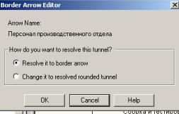
Rice. A2.24. Border Arrow Editor Dialogue

Rice. A2.25. Tunneling types of arrows

Tunneling can be used to depict insignificant arrows. If on any diagram of the lower level it is necessary to depict insignificant data or objects that are not processed or used by the works at the current level, then they must be sent to a higher level (to the parent diagram). If this data is not used in the parent diagram, it needs to be directed even higher, and so on. As a result, an insignificant arrow will be depicted at all levels and will make it difficult to read all diagrams where it is present. The exit is the tunneling arrow at the lowest level. This tunneling is called "not-in-parent-diagram".

Another example of tunneling can be a situation when the arrow of a mechanism migrates from the upper level to the lower one, and at the lower level this mechanism is used in the same way in all works without exception. (It is assumed that you do not need to detail the mechanism arrow, that is, the mechanism arrow on the child work is named before the fork, and after the fork, the branches do not have their own name). In this case, the arrow of the mechanism at the lower level can be deleted, after which it can be tunnelled on the parent diagram, and in the comment to the arrow or in the dictionary, you can indicate that the mechanism will be used in all works of the child decomposition diagram. This tunneling is called not-in-child-work (Figure A2.25).

Numbering of works and diagrams... All works of the model are numbered. The number consists of a prefix and a number. A prefix of any length can be used, but the prefix A is usually used. The context (root) work of the tree is numbered A0. The works i of the decomposition A0 have numbers A1, A2, A3, etc. The works of the lower level decomposition have the number of the parent work and the next serial number, for example, the work of decomposition A3 will have numbers A31, A32, AZZ, A34, etc. The works form a hierarchy where each job can have one parent and multiple child jobs, forming a tree. Such a tree is called a node tree, and the above numbering is called a node numbering. IDEF0 diagrams are double numbered. First, the diagrams are numbered by node. The context diagram always has the number A-0, the decomposition of the context diagram is number A0, the rest of the decomposition diagrams are numbers by the corresponding node (for example, A1, A2, A21, A213, etc.). BPwin automatically maintains numbering by nodes, that is, during decomposition, a new diagram is created and the corresponding number is automatically assigned to it. As a result of the examination, the diagrams can be refined and changed, therefore, different versions of the same (from the point of view of its location in the tree of nodes) decomposition diagram can be created. BPwin allows you to have only one decomposition diagram in a model at a given node. Older versions of the diagram can be stored as a paper copy or as an FEO diagram. (Unfortunately, when creating FEO diagrams, there is no rollback option, that is, you can get FEO decompositions from the diagram, but not vice versa.) In any case, you should distinguish between different versions of the same diagram. For this there is a special number - C-number, which must be assigned manually by the author of the model. C-number is an arbitrary string, but it is recommended to adhere to the standard when the number consists of an alphabetic prefix and a sequence number, with the initials of the author of the diagram used as the prefix, and the sequence number is manually tracked by the author, for example MCB00021.