Enterprise risk management (page 5)

Mathematical models of choice when making decisions under uncertainty are built on the basis of game theory.

Choosing solutions in the face of uncertainty includes:

Construction of a payment matrix (effects) and a risk matrix (damage or missed opportunities);

Quantify options.

The initial information for making decisions is the payment matrix (the matrix of consequences, the matrix of the game with nature).

Payment Matrix- statistical method of decision-making based on the choice of the best option from several alternatives according to pre-selected criteria.

View matrix , (3.1.)

called billing. Here Ai – option i-th solution ( i=1,.., m), Sj- situation or state of the environment ( j=1,.., n), ai j- the expected gain of the subject when choosing i-th solution and j

The elements aij payment matrices reflect the impact assessment (payments) for different options. The values ai j can be both positive (assessing the effect) and negative (assessing the damage).

A payment is a reward (utility) received as a result of the choice of a specific strategy Ai taking into account the specific circumstances Sj .

The payment matrix is ​​usually used in the following cases:

1) when the number of alternatives or strategy options is limited;

2) in the absence of complete certainty in the outcome of the chosen solution option;

3) when the results of the decision taken depend on the choice of the alternative and the circumstances that actually take place.

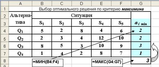
It is convenient to carry out the necessary calculations for choosing the optimal solution in the Excel environment. General view of the payment matrix with an additional row and two columns in which the largest a j max, a imax and the smallest a imin the value of the winnings is shown in Fig. 3.1.

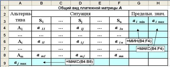
Rice. 3.1. Payment Matrix Layout in Excel

Each row of the matrix corresponds to one of the options for alternative solutions Ai, and each column is one of the possible situations Sj, which may arise for different values ​​of the decision maker's missing information about the conditions for solving the problem or about the expected results.

The player's task is reduced to the choice of such an option that would provide the greatest benefit in comparison with others.

In addition to this, the decision maker must have the ability to objectively assess the probability of relevant events (for which the result is consistent with the desired one) and calculate the expected value of such a probability. Situations of complete certainty (probability p- close to 1.0), or complete uncertainty (the probability is close to zero) are rare. Therefore, the decision maker in many cases has to independently assess the likelihood or the possibility of j-th event (conditions of partial uncertainty when 0<p<1,0) на основе анализа прошлых тенденций, своей субъективной оценки или собственного опыта действий в подобных ситуациях.

Accounting for probability directly affects the determination of the expected value in the payoff matrix. Failure to take into account the probability in the calculations leads to the choice of a solution with a more optimistic consequence.

When quantifying alternatives, two cases are possible.

1st case ... The probabilities of each j-th situations are determined by the results of processing statistical observations.

For each alternative, the mathematical expectation of the value of the alternative or strategy variant is determined, which is represented by the sum of the products of possible values a i j on the corresponding probabilities p j :

. (3.2)

Then an alternative option is selected A i, for which the mathematical expectation of a payoff is maximal, i.e. .

General view of the payment matrix with the probabilities of occurrence j-th situation is shown in Fig. 3.2.

Rice. 3.2. Payment Matrix Layout with Probabilities

2nd case ... Statistics on Probability Values pj are absent, then an expert assessment is made likelihood of occurrence j th situation.

Experts are offered three values ​​of the expected value S j characterizing the situation: optimistic, pessimistic and the most probable (modal). With the help of such triple estimates, the mathematical expectation of the predicted value is approximately determined, that is, the average probable value S cj... For binomial distribution, the following calculation formula can be used:

S cj = 1/6 [( S j ) min + 4( S j ) max]. (3.3)

Initial data can also be presented in the form of a risk matrix.

Risk matrix (matrix of missed opportunities) - a matrix, in the rows of which there are alternative variants of risk events, and in the columns - their probabilities and possible consequences (situations).

Quantifying the risk for each i-th solution for j-th situation is considered to be the difference between the maximum possible effect for this situation (aj ) max and its actual value a ij :

r ij = (aj) max -aij . (3.4)

Then the risk matrix is ​​written as follows:

, (3.5)

where r ij- the expected losses of the entity in the implementation of i-th solution option Ai (i=1,.., m) when implementing j-th variant of the state of the environment S j (j=1,.., n).

The optimal solution corresponds to the minimum mathematical expectation of risk:

, (3.6)

where pj- the probability of occurrence of the j-th situation.

Example 3.1. According to the well-known payment matrix (effects and damage)

it is necessary to build a risk matrix and choose an alternative solution without taking into account the data on the probability of individual situations and taking into account the expected values ​​of the probabilities of the implementation of a particular situation p1 = 0.10; p2 = 0.25; p3 = 0.30; p4 = 0.15; p5 = 0.20.

1. The elements of the payment matrix are entered into Excel and drawn up in the form of a table with the necessary comments, fig. 3.3.

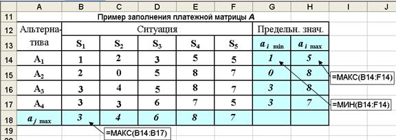
Rice. 3.3. Initial data, calculation formulas and calculation results

2. Using the built-in MAX function, the largest values ​​of the matrix elements are calculated for each j-th situation (a j) max: (a1) max = 3; (a2) max = 4; (a3) max = 6; (a4) max = 8; (a5) max = 7, according to which it is possible to establish the numbers of solution options corresponding to the maximum possible values ​​of the effect.

If the elements of the original matrix characterize the damage, then the opposite problem is considered with the calculation of the minimum amount of possible damage (MIN function) (a j) min: (a1) min = 1; (a2) min = 0; (a3) min = 3; (a4) min = 5; (a5) min = 5 and the subsequent determination of the corresponding number of the solution option (in Fig. 3.3, row a j min is not shown).

The same can be done with the estimates as much as possible (a i) max or minimum (a j) min of the possible effect (damage) for each i–Th solution option when the situation changes (see Fig. 3.3, the last two columns).

3. Risk estimates are calculated for each i-th solution for j-th situation using expression (3.4) and the risk matrix is ​​filled, Fig. 3.4.

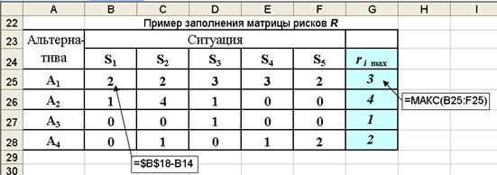
Rice. 3.4. Risk matrix and calculation formulas

4. From the alternative options, you can choose the optimal solution with the minimum risk value, it corresponds to option A3.

5. By expression (3.6), the risk of operations is calculated taking into account the probability of occurrence j-th situation and fill in the Risk column, Figure 3.5.

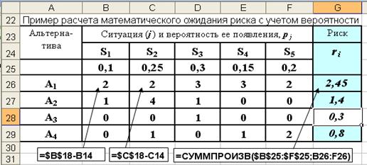
Rice. 3.5. Results of risk assessment of alternatives

Based on the results of the calculation (cells G26: G29), the optimal option A3 is selected, with a minimum mathematical expectation of risk equal to 0.3.

3.2. Choosing solutions in the face of uncertainty

When making a decision under conditions of uncertainty, the choice of a decision cannot be made either with the help of a deterministic or with the help of a probabilistic model, but you can use the categories of game theory.

External and internal factors influencing the choice of a decision when assessing the effectiveness of an investment are usually grouped into four groups:

Internal determinants - reflect the strengths of the investment project;

Internal uncertainties - reflect the weaknesses of the project;

External definite factors - characterize the opportunities provided by the external environment;

External uncertainties are considered as threats emanating from the external environment.

The main decision options are presented in the form of a decision matrix.

Decision matrix - a matrix of combinations of certain and uncertain factors that determine the effectiveness of investments, Figure 3.6.

When making decisions, an investor can find himself in one of four main situations.

State of the environment(situations)

Certain

external factors, P z

Undefined

external factors, N z

Strategies

Certain

internal factors

P w

Strategy 1

maximax

( maxmax )

P w « P z

Strategy 4

minimax

( minmax )

P w « N z

Undefined

internal factors

N w

Strategy 3

maximin

( maxmin )

N w « P z

Strategy 2

minimina

( minmin )

N w « N z

Figure 3.6. Decision matrix

Strategy 1.P w « P z The investor is in a favorable situation, he has investment potential and can realize his investment opportunities, since the environment creates favorable conditions for this. With this in mind, the investor should maximize the use of his opportunities and choose a strategy maximax.

Strategy 2.N w « N z . The investor is in the worst situation, as external threats are amplified by the internal weaknesses of the enterprise implementing the investment project. In such conditions, it is necessary to minimize these weaknesses and threats, that is, to apply the strategy minimina... Such a strategy, in a pessimistic version, leads to abandonment of the project, and in an optimistic version, to a desire to survive an unfavorable situation.

Strategy 3.N w « P z . External opportunities are difficult to use due to the weaknesses of the investment project itself (or due to the unsatisfactory state of the enterprise itself). In this case, the strategy is chosen maximin, which should be aimed at minimizing weaknesses in order to use external opportunities.

Strategy 4. P w « N z . Internal investment opportunities aimed at enterprise development are subject to external threats. The investor must apply the strategy minimax, that is, to resist the difficulties that the environment creates for him, in order to maximize his inner potential.

Strategies can be: economic indicators of the state of the enterprise, various options for solving the assigned tasks, technical parameters of the designed systems, etc.

The factors characterizing the state of the environment may include: the level of demand for goods offered by the firm, market prices, operating conditions of technical and production systems, actions of competitors, etc.

The choice of strategy in conditions of uncertainty of possible probabilities of the situation is made on the basis of special criteria in the form of non-stochastic models, which include the following criteria: rationality criterion; maximax criterion; maximin test; minimax criterion, etc.

3.3. Criteria for Choosing Decisions in Conditions of Partial Uncertainty

The previously considered situations of maximizing the average expected income (3.2) and minimizing the average expected risk (3.6) with a known probability p j the fact that the real situation develops according to the option j are called partial uncertainty... Laplace's criterion can be added to the same cases.

Lapplepasse criterion of rationality (equal opportunity, indifference) based on the principle of equal probabilities ( pj = 1/n) for all variants of a real situation.

When using the criterion of maximizing the average expected income, a solution is selected that achieves

, (3.7)

where qij- expected income when choosing i-th solution and j-th state of the environment (situation).

In the case of minimizing the average expected risk, a solution option is selected for which

. (3.8)

r ij- expected losses when choosing i-th solution option and implementation j-th variant of the state of the environment.

Example 3.2. Using the Laplace criterion of equality for the input data given in the consequences matrix

,

it is necessary to choose the best solution based on: a) the rules for maximizing the average expected income; b) rules for minimizing the average expected risk.

a) Taking into account the equal probability of five options for the outcome of a real situation ( pj= 1 / n = 1/5), the values ​​of the average expected income for each of the solution options are estimated by expression (3.2) and are = 5, = 6.2, = 7.00, = 4.4 (Figure 3.7).

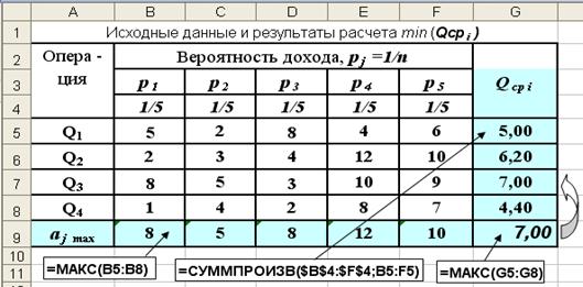
Rice. 3.7. The results of calculating the average expected income

According to Laplace's criterion (3.7), the best solution would be the third, with the maximum average expected income equal to = 7.00.

b) The elements of the risk matrix are calculated by expression (3.4) and for each solution option by expression (3.6) the values ​​of the average expected risk are calculated taking into account the equiprobability of the situations: = 3.60, = 2.40, = 1.60, = 4, 20 (Figure 3.8).

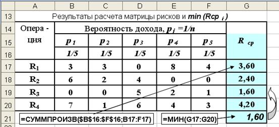
Rice. 3.8. Matrix of risks and values ​​of the average expected risk

Taking into account Laplace's criterion (3.8), the third option will be the best, with the minimum value of the average expected risk equal to 1.60.

3.4. Criteria for Choosing Decisions in Conditions of Complete Uncertainty

Maximax criterion (extreme, "pink" optimism) is based on the optimistic principle of L. Hurwitz, according to which the option is selected that provides the greatest effect in the most favorable situation.

If the consequences matrix (3.1) is considered as the effect matrix E,

. (3.9)

This criterion corresponds to strategy 1 (see Figure 3.6), it is advisable to apply it in cases where it is possible to influence the opposite side in order to make the uncontrolled external environment more favorable, and to realize the possibilities of optimal use of controlled internal factors.

Example 3.3. Taking the matrix of consequences in example 3.2 as the matrix of effects, choose a solution option according to the maximax criterion.

1. The initial data is entered into Excel (Fig. 3.9). Then, using the MAX function for cells (B4: F4;…; B7: F7), the maximum values ​​for each solution are sequentially found: a1 =8, a2 =12, a3 =10, a4 =8 .

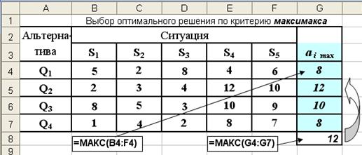
Rice. 3.9. Results of choosing the optimal solution according to the maximax criterion

2. From the sequence of found maximum values ai(G4: G7) The MAX function (cell G8) selects the largest value: a2 =12 , with this in mind, it is recommended to make a second decision.

If the elements of the matrix A (3.1) are the costs Z, then they can be considered as losses, and then the solution providing the lowest costs is selected from the conditions for minimizing costs:

. (3.10)

Minimin criterion (pessimism) is based on the pessimistic principle, according to which, in an unfavorable external environment, controlled factors can be used in an unfavorable way. Then, if the consequences matrix is ​​the effect matrix E, then the effective solution is selected from the conditions for ensuring the maximum:

. (3.11)

In real conditions, it is not always possible to control the uncontrollable factors of the external environment, especially when it is necessary to take into account the time factor. For example, with long-term forecasting and planning; design of complex objects, etc. Or, for example, production costs are controllable factors in short time intervals and uncontrollable in the long term, since the cost of electricity, the cost of materials and purchased products, etc. are not known in advance.Another example is the determination of the volume of production of an enterprise ( controlled factor), which depend on various factors associated with the production process. These factors relate to the internal environment of the enterprise: the level of design and technological preparation of production, the type of equipment used, the qualifications of workers, etc.

This criterion corresponds to strategy 2 (see Figure 3.6).

Example 3.4. Taking the matrix of consequences in example 3.2 as the matrix of effects, choose a solution option according to the minimin criterion.

1. The initial data is entered into Excel (Fig. 3.10). Then, using the MIN function for cells (B4: F4;…; B7: F7), the minimum values ​​for each i-th solution: a1 =2, a2 =2, a3 =3, a4 =1 .

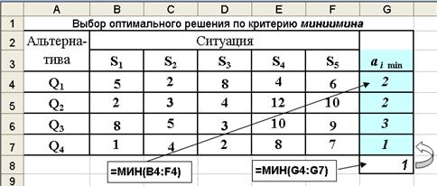
Rice. 3.10. Results of choosing the optimal solution according to the minimin criterion

3. From the sequence of found minimum values ai(G4: G7) Use the MIN function (cell G8) to select the smallest value: a4 =1 , with this in mind, it is recommended to make a fourth decision.

When analyzing the cost matrix, the pessimism criterion takes the following form

(3.12)

Maximin criterion (extreme pessimism) based on the pessimistic principle of A. Wald, according to which the option is chosen, the result of which is the most favorable among the least favorable.

If the expected situation develops unfavorably, that is, will bring the smallest income: ai= min ai j, then such a solution is chosen for which the minimum (guaranteed) income turns out to be the greatest

. (3.13)

This criterion is conservative, since it offers a choice with a cautious line of behavior, therefore it is advisable to use it in cases where it is necessary to ensure success under any possible conditions. In the decision matrix (Figure 3.6), Wald's criterion corresponds to strategy 3.

Example 3.5. For the consequences matrix in Example 3.2, choose a solution option based on the maximin criterion.

1. For each i–Th alternative solution, using the MIN function, the minimum values ​​are found: a1 =2, a2 =2, a3 =3, a4 =1 (see figure 3.11, cells G4: G7)

Rice. 3.11. Results of choosing the optimal solution according to the maximin criterion

2.Using the MAX function from the sequence of found minimum values ai(G4: G7) the maximum a3 = 3 (cell G8).

3. According to Wald's rule (3.11), preference should be given to the third solution ( i=3 ), with the maximum guaranteed result (gain) regardless of the variant of the situation (external conditions).

Minimax criterion (minimax risk, expectation of losses) based on L. Savage's frustration principle. According to this principle, an option is selected, in the implementation of which the maximum possible disappointment (the difference between the maximum possible result and the results that can be obtained for each of the remaining options) turns out to be the smallest.

Here they are guided by the worst situation, which is associated with the greatest risk. When choosing a solution, a risk matrix is ​​used R(3.5). The best solution is the one in which the maximum risk value is the smallest:

. (3.14)

When making investment decisions under conditions of uncertainty with a focus on the worst outcomes, the pessimistic criterion (maximin) and the criterion of disappointment (minimax) are applied.

This criterion is used in cases when it is required to avoid a large risk in any conditions; it corresponds to strategy 4 (Fig. 3.6).

Example 3.6. Using the consequences matrix in example 3.2, choose a solution option based on the minimax criterion.

1. Preliminarily, according to the matrix of consequences of example 2, using expression (3.4), the elements of the risk matrix are calculated in Fig. 3.12.

2. In each row of the risk matrix, using the MAX function, its maximum element is selected (cells G4: G7): ri = : r 1 = 8, r 2 = 6, r 3 = 5, r 4 = 7.

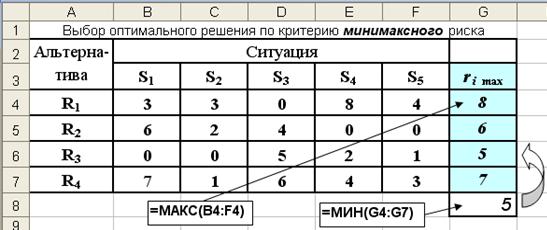
Rice. 3.12. Results of choosing the optimal solution according to the minimax criterion

3. According to Savage's rule, the smallest of these values ​​is selected (MIN function in cell G8): r 3 = 5, that is, the 3rd decision should be made ( i=3 ). The choice of this option means that the maximum losses under various scenarios of the situation will be minimal and will not exceed 5 units.

Hurwitz criterion for generalized maximin (pessimism-optimism) presupposes a choice mixed strategy when, in a certain proportion, pessimism (caution) and optimism (propensity to take significant risks) are combined, that is, an intermediate decision is chosen between the line of behavior in view of the worst and the line of behavior in view of the best.

According to this criterion, a solution option is selected, at which the maximum indicator is achieved G defined from the expression:

Gi = max[a minai j + (1 - a) maxai j]. (3.15)

i j j

where butij- the payoff for i-th solution for j-th variant of the situation,

a- coefficient reflecting the degree of optimism ( 0 ≤ a ≤ 1 ): at a = 0 a line of behavior is chosen with the expectation of the best, that is, an orientation towards the marginal risk is made (we obtain the maximax criterion); at a = 1 focus on the worst, then we get the Wald criterion - a guideline for cautious behavior. Intermediate values a between 0 and 1 and are chosen depending on the specific situation and the risk appetite of the decision-maker.

Example 3.7. The enterprise is preparing to release new types of products, while four solutions are possible Q 1, Q2 , Q3 , Q4 , each of which corresponds to a certain type of product or their combination. The structure of demand for products is characterized by three scenarios S 1 , S 2 , S 3 ... Efficiency of the release of new types of products buti j for each pair of solution combinations Qi (i=1,2,…, m) and the setting S j (j=1,2,…, n) are given in the table in Figure 3.12. It is necessary to find the most profitable solution according to the Hurwitz criterion Qi and to evaluate the influence of the optimism coefficient on the choice of the solution.

1. Let us set the sequence of coefficients k with a step of 0.25: 0; 0.25; 0.50; 0.75; 1.00 and enter the initial data on the Excel worksheet, fig. 3.12.

2. The results of calculating the indicator G by expression (3.13) for various solutions depending on the value of the coefficient k are shown in the bottom table in Figure 3.13.

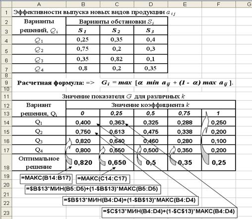
Rice. 3.13. Initial data, calculation formulas and calculation results of the Hurwitz criterion (arrows show effective solutions)

As can be seen from the figure (cells B18: F18), the change in the coefficient k influences the choice of a solution that should be preferred.

The choice of this or that criterion depends on a number of factors:

The nature of the problem being solved;

The set goals,

Sets of restrictions

Risk appetite of decision-makers.

It should be noted that the considered methods and techniques for solving problems in conditions of risk and uncertainty are not limited to the listed methods. Depending on the specific situation, other methods can be used in the analysis process, for example, using the standard deviation and the coefficient of variation as a measure of risk.

3.5. Analysis of profitability and risk of financial transactions based on the Pareto optimality principle

A financial operation is called a transaction, the initial and final states of which have a monetary value, the purpose of which is to maximize income - the difference between the final and initial estimates.

Usually, financial transactions are carried out in conditions of uncertainty and therefore their outcome cannot be predicted in advance. Therefore, financial transactions are risky, that is, when they are carried out, both profit and loss are possible (or insignificant profit compared to the expected one).

There are several ways to assess a financial transaction in terms of its profitability and risk. Most often, the income of a transaction is presented as a random variable. Q, and the risk of surgery r is estimated by the standard deviation of this random income.

General formulation of the problem. Let be BUT - some set of operations that differ in at least one characteristic. When choosing the best operation, it is desirable that Q there was more, but r less.

Consider that the operation but dominates operation b ( denoted a> b), if Q (a) ≥ Q (b) and r(a) ≤ r (b) and at least one of these inequalities is strict. In this case, the operation but called dominant, and the operation b – dominated. Moreover, no dominated operation can be recognized as the best, therefore the best operation should be sought among the non-dominated operations. A lot of non-dominated operations are called set (area) Pareto or Pareto optimality set.

For the Pareto set, the following statement is true: each of the characteristics Q,r is a single-valued function of the other, that is, on the Pareto set, one can uniquely determine the other by one characteristic of the operation.

Example. 3.8. Of the four possible financial transactions with expected returns Q 1, Q 2, Q 3, Q 4 and the corresponding probabilities of obtaining them p1, p2, p3, p4 it is necessary to choose the Pareto optimal operation.

Values ​​of expected returns qj and their corresponding probabilities pj are given in the following matrix

p1 p2 p3 p4

Since the expected income of a financial transaction is considered a random variable Q, then its average value is estimated by the mathematical expectation: , (3.16)

where pi j- the likelihood of earning income qi j in i- oh financial transaction.

A quantitative measure of risk r financial transaction is considered s - standard deviation

r i = , (3.17)

which characterizes the degree of dispersion of possible values ​​of income around the average expected income. It is convenient to estimate the dispersion of the yield D by the formula: D [ Q i] = M [( Q i-) 2] = M [ Q i 2 ] – .

Here M [ Q i 2 ] = å q 2 i jpi j Is the mathematical expectation of the square of the expected return in i th financial transaction.

Calculations of the average expected income and risks using the above formulas will be performed in the Excel environment. Worksheet with initial data, calculation formulas and the results of calculating average returns Q c p and risk r is shown in Fig. 3.14.

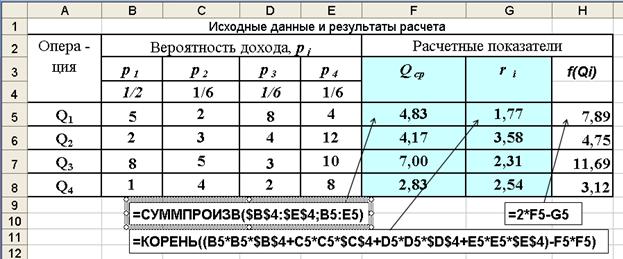
Rice. 3.14. General view of the worksheet with the calculation results

The average expected incomes found as a result of the calculation Qi and the associated risks ri plot on the graph in the coordinate system: income (vertical axis) - risks (horizontal axis), Fig. 3.15.

Rice. 3.15. Graphical interpretation of the results of calculating the efficiency of financial transactions in the coordinate system: expected profitability - risk

Let's analyze the relative position of 4 points on the chart from the point of view of their dominance. The higher the point (`Q, r), the more profitable the operation, the more the point to the right - the more risky the operation. This means that you need to choose a point above and to the left. A point (`Q ¢, r ¢) dominates a point (` Q, r) if `Q ¢ ³`Q and r ¢ £ r. In this case, the 1st operation dominates the 2nd, the 3rd dominates the 2nd and the 3rd dominates the 4th. But the 1st and 3rd operations are incomparable - the profitability of the 3rd is higher, but its risk is also greater.