A perfectly competitive firm gets it in the long run. A market of perfect competition. Equilibrium in the short and long term

Perfect competition and its characteristics

Depending on the structure, the market can be a market of perfect competition, a market of monopolistic competition, monopoly and oligopoly.

Definition 1

Perfect competition is a type of market structure that is characterized by the presence on the market of many (usually large) firms producing homogeneous products, relatively simple entry and exit from the market, as well as a high level of availability of information about the state of the market to all its subjects.

This type of market structure has the most ancient origin, while it is the simplest and most understandable in terms of pricing, the basis of which is provided only by the interaction of market supply and demand. This pricing mechanism is most suitable for determining the costs of production and sales, profitability and profitability of the organization.

A characteristic feature of the perfect competition market is a standardized product with homogeneous consumer properties. The presence of such a product ensures that the buyer is indifferent to trade marks; he does not care from which manufacturer to buy the product. As a result, the price, the value of which is determined by the market, is the only significant criterion for choosing a product. The pricing process is determined by the essence of the market mechanism, in which the price is formed by establishing an equilibrium between market supply and demand.

At the same time, each specific manufacturer does not take part in pricing, but follows the price that has already formed in the market in a natural way.

The demand for a product of a specific shape is shown by a straight horizontal line.

The indicators of the firm's income are determined by the following formulas.

Total (cumulative):

$ TR = P \ cdot Q $, where:

• $ TR $ - total revenue, monetary units;
• $ P $ - the price of the good (price), monetary units;
• $ Q $ - realized quantity of goods (quantity), units.

Average:

$ AR = \ frac (TR) (Q) = \ frac (P \ cdot Q) (Q) = P $

where $ AR $ is the average revenue, in monetary units.

Limit:

$ MR = \ frac (∆TR) (∆Q) = \ frac (∆ (P \ cdot Q)) (∆Q) = P \ cdot \ frac (∆Q) (∆Q) = P $

where $ MR $ is marginal revenue, in monetary units.

Regardless of the volume of additionally produced products, the firm has no opportunity to influence the price of the goods. As a result, the sale of any additional unit of goods is carried out at the same price as those preceding it.

Features of perfect competition in the long run

The long-term period is defined as the time sufficient for a firm to enter and exit the industry.

The long-term period of perfect competition is characterized by the special interaction of supply and demand of a competitive firm.

Under these conditions, the demand curve of such a firm acts as a characteristic of the volume of products produced at each price level to achieve the maximum profit in the long run.

The long-term range of a competitive firm's supply curve is represented by the portion of the $ LMC $ curve above $ LACmin $, which is the long-term break-even price.

Figure 1. The ratio of supply and demand. Author24 - online exchange of student papers

Definition 2

The long-term break-even price is the minimum price that provides the firm with cost coverage only in the long run.

Getting a firm in the long run of high profits is a factor that attracts other participants to the market. The resulting increase in sales leads to a decrease in the price of the product and the displacement of small firms with non-technological production from the market. The fluctuations will stop when the price of the commodity reaches the $ LACmin $ level. At this point, the market will lose its attractiveness to new firms, since the firms operating in the market will receive zero profits. That is, firms that have already mastered the market by that time will have accounting, but not economic (including implicit costs) profit. As a result, these firms will have no incentive to exit the market, while new firms will have no incentive to enter.

In the long run, equilibrium will be established in the industry, which is expressed in the absence of firms' desire to leave the industry, to enter it, to increase or decrease production volumes.

A competitive market in the long term is characterized by three main points:

• first, the coincidence of supply and demand in the market, providing an equilibrium price that suits both sellers and buyers;
• secondly, the finding of all firms in the industry in an equilibrium position that provides them with the maximum profit;
• thirdly, the receipt of zero profit by all firms.

The creation of such conditions requires a long period of time, in a short period firms have the opportunity to obtain high economic profits.

Experts note the presence of a profit paradox: the receipt of economic profit in the industry, the value of which exceeds zero, acts as an incentive to attract new firms to enter the market. An increase in the number of sellers ensures an increase in supply, which leads to a decrease in prices and the establishment of a new equilibrium in which the value of economic profit reaches zero. In this way, firms achieve equilibrium in the long run, earning zero profit, which leads to a lack of desire to enter or exit the industry. This moment characterizes the achievement of production efficiency by the company.

In the long run, the determination of the market supply is carried out by summing the supply of all firms operating on the market. The graphical expression of the supply curve in the long run depends on the dynamics of the level of costs under the influence of an increase in production. This factor determines the positive or negative slope of the curve. With absolute elasticity of supply and, as a consequence of the independence of average costs from the number of firms in the market, the supply curve takes a horizontal position.

The long-term supply curve depends on changes in the long-term level of the industry's costs as the volume of output expands. Depending on this, it has a positive or negative slope. If the average costs do not change depending on the change in the number of firms in the industry, the supply of the industry is absolutely elastic, the supply curve is horizontal.

In the long run, firms are able to make changes in their activities that are not available in the short run. In the short term, a certain number of firms operate in the industry, each of which has constant, unchanging production capacities. Indeed, firms may close in the sense that they will produce zero units in the short run; but they don't have enough time to liquidate their assets and go out of business. In contrast, in the long run, firms already in the industry have ample time to either expand or contract their production capacity. In addition, it is important that the number of firms in an industry can either increase or decrease as new firms enter the industry or existing firms leave it.

Rice. 2.2. The position of a competitive firm in the long run

The long-term time frame assumes the mobility of all production resources. After all long-term adjustments have been completed, the product price and production volume will exactly match the minimum average cost. This conclusion follows from two main factors: 1) firms strive for profits and beware of losses; 2) in conditions of perfect competition, firms freely enter and leave the industry. If the initial price is higher than the average total cost, then the opportunities for generating economic profit will attract new firms to the industry. This expansion of the industry will increase the supply until the price drops again and equals the average total cost. Conversely, if the price is initially below average total costs, the inevitability of losses will cause a number of firms to exit the industry. As a result, the aggregate supply will decrease, which will lead to an increase in prices to the minimum value of the average total costs.

As you enter the industry, the supply of a product on the market will increase, lowering its price. Economic profits will persist, and therefore firms will enter the industry until short-term market supply increases. Then the market price, and hence the marginal revenue of the firm, will decline. The economic profit generated by increased demand is reduced by competition to zero, after which the powerful incentive that has prompted many firms to enter the industry disappears. Long-term balance is restored.

Rice. 2.3. Temporarily earned profit and restoration of long-term equilibrium of (a) a firm that is a representative of the industry and (b) the industry as a whole

Falling consumer demand leads to lower prices, making production unprofitable with minimal average total costs. The resulting losses will eventually force firms to leave the industry. The reason is that somewhere else, owners may be making normal profits, as opposed to below-normal profits (losses) that they now face. However, as some firms exit, the sectoral supply will decrease, and the price will rise. As a result, the break-even point is reached, and, therefore, the industry is again in a position of long-term equilibrium.

Rice. 2.4. Temporarily existing losses and restoration of long-term equilibrium of (a) a firm that is a representative of the industry and (b) the industry as a whole

CONCLUSION

Economists group different industries based on their market structure. There are four market structures: perfect competition, absolute monopoly, monopoly competition and oligopoly.

A highly competitive industry consists of a large number of independent firms producing a standardized product. Perfect competition assumes that firms and resources can easily move from industry to industry.

In a competitive industry, no firm is able to influence the market price. The demand curve for the firm's product is perfectly elastic, and the price is therefore equal to marginal revenue.

Read other articles on economics

Economic and statistical analysis of grain production
Crop production is one of the main branches of agricultural production. The national economic importance of plant growing is enormous and is primarily determined by the fact that it provides a person with almost all products of plant origin. Crop production is ...

Share capital and its structure
Share capital is the source of financing for the company and is reflected in passive accounts. ...

Short term such a period is called, in the course of the cat, the production capacity of the company is fixed, but the volume of output can be changed (increased, decreased) by changing the volume of using a change of factors. The total number of enterprises remains unchanged.

The purpose firms is profit maximization.

Profit () is the difference between scoop income ( TR) and scoop costs ( TS) firms: P r = TR- TS.

Both the scoop of income and the scoop of the company's costs are the function of output Q... Since the market price is not under the control of a competitive firm, its main the task of composition in determining the optimalVrelease, with the cat she can maximize profits.

Equilibrium release there is the volume of production, with the cat the profit of the company is maximum.

There are 2 methods for determining the optimal V output, when a competitive firm will maximize profits:

1) the method of comparing the scoop of income and the scoop of costs ( TR and TS);

2) the method of comparing the limit of income and the limit of costs ( MR and MC).

When using the second method, 2 values ​​are determined and compared: marginal revenue (MR) and marginal cost (MC).

As long as marginal revenue exceeds marginal cost ( MR > MC), the company should expand production, because, having increased V production by units, the company has its profit. It should be remembered that the firm is interested in the profit for the entire mass of the output (and not only for the marginal unit). But as soon as the pre-e costs exceed the marginal income ( MR < MC), the firm should reduce production, otherwise its profits will decline.

So, a competitive firm will maximize profits or minimize losses by producing suchVpr-tion, when the marginal income is equal to the marginal cost(fig. 14):

MR = MC.

Equality MR and MC was the condition for maximizing profits for any firm, regardless of the market structure in which it operates.

Since for a market of perfect competition MR = P, then this equality will take the form:

MR = P = MC.

The firm made a profit when the income per unit of production, i.e. AR, exceeds the cost of a unit of production, i.e. AS... But since AR = P, then this is tantamount to the assertion that the firm makes eq profit every time when the market price of the commodity exceeds cp total costs, i.e. R > AS.

In the short term, all firms will be divided into 4 groups:

firms that receive positive eq profit;

firms that receive normal profits (zero eq profit);

firms that minimize losses;

firms terminating production.

Firm supply curve in the short term - This is an expression of the relationship between the market price and the volume of the offered goods (Fig. 15).

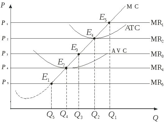
At a price R 1 and V issues Q 1 firm receives economic profit , because R 1 > ATC... At a price R 2 and production volume Q 2 the firm receives normal profit (all costs are reimbursed), since R 2 ATC... Point E 2 call break-even point. At a price R 3 and V issues Q 3 firm minimizes your losses , since ATC> R 3 > AVC... At a price R 4 and the volume of production Q 4 firm carries losses equal to its fixed costs , because R 4 > AVC... The firm is indifferent - to produce pr-tion or to close. Point E 4 call closing point. At a price R 5 and the volume of issue Q 5 firm will not produce, because R 4 = min AVC.

Since at the price R 1 , R 2 , R 3 , R 4, the firm will carry out the release of the pr-tion, and at a price R 5 prefers closing, then the following conclusion can be drawn: The supply curve of a perfectly competitive firm focused on maximizing profits in the short run coincideswith the ascending part of the MC curve lying above the point min AVC.

The short-term supply curve discussed above describes the prompt response of a profit-maximizing or loss-minimizing firm to short-term, current fluctuations in the price of a commodity. However, the entrepreneur is interested not only in the immediate result, but also in the prospects for the development of the enterprise. The main strategic criterion is to obtain a stable stream of profits through active access to the most efficient production volumes in accordance with the forecast of the market in the long term.

If a firm has an economic profit in the short run, its production becomes more attractive to other manufacturers. New firms enter the market for this product, diverting part of the effective demand to themselves. In order to successfully sell, this enterprise is forced to reduce prices or incur additional costs to support sales. Profits are falling, the influx of competitors is decreasing. In the case of unprofitable production, the picture is the opposite. Individual firms will be forced to leave the industry, which will increase the demand price for the rest of the firms. This process will continue until the price covers the average costs of the remaining firms in the industry, i.e. while P = ATC... if the process of exit of firms from the industry continues, then the rise in price will lead to its rise above the average costs for firms remaining in the industry and to the receipt of economic profit by these firms. But these profits, in turn, serve as a signal for new firms to enter the industry. The process of entering and exiting will only stop when there is no economic profit. When a firm makes zero profits, it has no incentive to go out, and other firms have no incentive to go in.

Economic profit will correspond when the price coincides with the minimum of long-term average costs ( LAC), i.e. the firm will be of the "marginal" type.

Thus, the condition for the long-term equilibrium of the firm will be the equality of the price to the minimum of long-term unit costs, i.e. P = min LAC(fig. 5).

Production at the lowest average cost means producing with the most efficient combination of resources, i.e. firms use factors of production and technology in the best possible way. This is undoubtedly a positive phenomenon primarily for the consumer. It means that the consumer receives the maximum volume of products at the lowest price that the unit costs allow.

Figure 5 - Equilibrium of the firm in the long run

The firm's long-run supply curve, like the short-run supply curve, is part of its long-run cost curve ( MC), located above the minimum point of long-term unit costs - point E... If the price falls below the minimum point for long-run unit costs, the firm does not cover all costs, so it should leave the industry.

The market supply curve will be obtained by summing the volumes of long-term supply of individual firms. However, in contrast to the short term, the number of firms may change in the long term.

In this regard, three options for changing the industry supply are possible:

• 1. the offer price is unchanged;
• 2. the offer price increases;
• 3. the offer price decreases.

The implementation of this or that option is determined by the degree of dependence between the change in the volume of output and the change in the supply price. The level of the supply price, in turn, is determined by the amount of costs and, therefore, the cost of resources.

1. The offer price will remain constant if resource prices do not change. The latter is possible in the case when the demand for resources of a particular industry makes up an insignificant part of the total demand. The industry can expand without significant impact on prices and costs. The expansion and contraction of the industry only affects the volume of production and does not affect the price.

An increase in demand means moving the corresponding curve upward to the right, towards a higher price, since any firm in the industry is in the position of a price receiver, it will consider an increase in price as an external factor and will react to it by increasing the volume of production with Q 1 before Q 2 ... Attracting new firms into production and tightening the competition regime will lead to an increase in market supply up to Q 3 and lowering the price to the original level. Thus, the long-term equilibrium of the firm will be restored, and the supply curve of the industry will be a completely horizontal line.

This is the case of the fixed cost industry. Typically, we are talking about the use of traditional resources used by many other industries.

• 2. The offer price will increase if the resource prices increase. Most industries use specific resources, the amount of which is limited. Their application determines the upward nature of the costs of a given industry. As the industry expands, the average cost curves shift upward. The entry of new firms increases the demand for resources and raises the price. Therefore, the industry will produce more products only at a higher price (Figure 6, b). This is an industry with increasing costs.
• 3. The offer price will decline if the resource prices decrease. The long-term supply curve will have a negative slope. As the industry grows larger, it becomes possible, due to its size, to acquire a large number of factors of production at a lower price. In this case, the curves of average costs of firms shift downward and the market price of the product decreases. The decline in the market price and average costs leads to a new long-term equilibrium of the industry with a large number of firms, with a large volume of production and with a lower price for products. Consequently, in an industry with declining costs, the industry's long-run aggregate supply curve slopes downward.

In any case, in the long run, the industry's supply curve will be flatter than the short-term supply curve. This is due to the fact that, firstly, the ability to use all resources in the long run allows you to more actively influence the price change. Therefore, for each individual firm, the supply curve will be more elastic. Second, the ability of new firms to enter the industry and to leave the “old” industry allows the industry to respond to changes in market prices to a greater extent than is possible in the short term. Accordingly, output will increase or decrease by a greater amount in the long run than in the short run in response to an increase or decrease in price. In addition, the lowest point in the industry's long-term supply price will be higher than the lowest point in the short-term supply price, since all costs are variable and must be recovered.

Based on all of the above, the basic equilibrium positions of a perfectly competitive firm are as follows:

• · Perfect competition is a special form of market organization, the main feature of which is the inability of the manufacturer to influence the market price;
• · The main motive of the activity and the criterion of the equilibrium of the manufacturer is the maximization of profits or the minimization of losses;
• · Should distinguish between the behavior of a perfectly competitive firm in the short and long run;
• · In the short run, the firm optimizes the volume of production, proceeding from the equality of prices to marginal costs. If at the same time the price is equal to the minimum of average variable costs, it is advisable to close production;
• · In the long run, the company optimizes the scale of production, proceeding from the equality of the price to the minimum of long-term unit costs;
• · The supply of goods on the market as a whole consists of the proposals of individual manufacturers.

In the presence of competition in the market, manufacturers constantly strive to reduce their production costs in order to increase profits. As a result, productivity increases, costs decrease and the company is able to reduce retail prices, thus increasing production efficiency, competition leads to lower prices.

6.2. Perfect competition. Equilibrium in the short and long term

The market in conditions of perfect competition has the following features:

1. A large number of firms operate in this market, each of which is independent of the behavior of other firms and makes decisions independently. Any firm in the industry is unable to influence the market price of the goods produced by the industry.

2. Firms of the industry produce one and the same (homogeneous) product, therefore for buyers it is absolutely indifferent which product of which firm to purchase.

3. The industry is open to entry and exit of any number of firms. Not a single company in the industry takes any resistance, as there are no legal restrictions to this process.

Individual firm demand. Since, in conditions of perfect competition, the firm of the industry, within the boundaries of changes in the volume of its output, does not have a significant effect on the price of goods and sells any quantity of goods at a constant price, the demand for the products of an individual firm is absolutely elastic, and the demand curve of each firm is horizontal. In addition, each additionally sold unit of goods will add the same amount of marginal revenue equal to the price of the goods to the total revenue of the firm.

Consequently, for an individual firm operating in a perfectly competitive market, the average and marginal revenue are equal to the price of goods P, i.e. MR = AR = P, therefore the curves of demand, average and marginal revenue coincide and represent the same horizontal line drawn at the level of the price of the product.

Equilibrium in the short and long term

According to rules 1 and 2 (see Topic 6.1), operating in each market structure, a firm, in order to maximize profits, must produce such a volume of goods and services. q E at which MR = MC(rule 2) and P> AVC(rule 1). But in conditions of perfect competition, the marginal revenue MR is equal to the average revenue AR and the price of the product, i.e. MR = AR = P.

This means that, operating in a perfectly competitive market, a firm will maximize profit if it produces such a volume of q goods at which marginal costs are equal to the price of a good set by the market regardless of the firm's actions.

This situation is reflected in Fig. 13.

Rice. 13. Equilibrium in the short run

By producing Qe units of a commodity when MC = P, the firm maximizes profits, and any deviations from this volume reduce its profits. If the firm will release Q1< Qe единиц товара, то цена товара (которая не меняется) станет превосходить предельные издержки, и фирма обязана в этих условиях увеличить производство, иначе она не максимизирует прибыль. Когда же Q2 >Qе, marginal costs begin to exceed the price and the firm needs to reduce the volume of output.

Note that at point E1 the marginal costs MR are also equal to the price of goods P, but at point E (not E1) the price P exceeds the average variable costs AVC, i.e. Rule 1 is satisfied. Hence, it is at point E, not E1 that the firm has an equilibrium in the short run.

Supply curve in the short run. The market price of the product. Suppose that the initial price P under the influence of the market has increased to P e1. As has just been shown, under these conditions the firm will increase its output to such a level Q e1, when the marginal cost is again equal to P e1. Therefore, for any price Pi that exceeds AVC, the firm will produce so many units of the good that the marginal cost MCi corresponding to this volume of production equals Pi. But since the MC curve shows the value of marginal costs for any values ​​of Q, the points of the MC curve and will determine the production volumes at all values ​​of the price when MC = P. In addition, according to rule 1, if the price of a product falls below the AVC value, then the firm will stop existence and Q = 0. But, as you know, the curve showing the ratio of the price of a product to the number of units offered by the firm for sale is the supply curve.

An important conclusion follows from this: the supply curve of a firm operating in the short run in perfect competition is the segment of the marginal cost curve above the AVC curve(segment VC in Fig. 13).

If there are N firms in the industry, supply curves can be similarly constructed for each of them. Then the supply curve of an industry can be obtained by horizontal summation of the supply curves of individual firms.

The market price of a product in perfect competition is determined by the intersection of the industry supply curve and the market demand curve. Although each firm in the industry does not significantly affect the market for a product, the joint actions of all firms in the industry (as reflected by the supply curve of the industry), as well as collective actions of households (as reflected in the market demand curve) can lead to displacements of supply and demand curves and changes in the equilibrium price. ... But at a new equilibrium price, each firm will strive to produce so many units of a homogeneous product that MC = P. At such volumes of output, the QS of the industry equals the market QD, and equilibrium occurs in the industry.

However, for the company, the amount of profit it makes is of great importance. The firm makes a profit if the revenue per unit of production, i.e. AR, exceeds the cost per unit of production, i.e. ATC. But since AR = P, then this is tantamount to the statement that the firm makes an economic profit whenever the market price of the product exceeds the average total costs, i.e. when P> ATC... This means that, depending on the value of the market price of the product, three options are possible.

1. The price of the goods is lower than the average total costs for the volume of production q, when MC = P; in this case, the firm will have losses (Fig. 14a).

2. With the volume of production q, the price of the goods coincides with the value of the average total costs and the economic profit is equal to zero. The volume of output in this case reflects the so-called break-even point (Fig. 14b). The level of instability is observed when the total costs are equal to the total revenue ТС = TR or when the marginal and average costs are equal (MC = ATC).

3. The price of the product is higher than the average total costs for the release of q units of the product; in this case, the firm will make a profit (Fig. 14 c).

Rice. 14. Possible options for equilibrium in the short term

Consequently, the firm, predicting its activities, must determine the production volumes at which the minimum values ​​of ATC and AVC are achieved. They will serve as a guideline for the behavior of the company in a given market structure, allowing you to find the break-even level and the moment of termination of production.

Long-term balance

Over the long term, firms can adapt to various changes in the market. For a long-term period in a perfectly competitive market, the following conditions are characteristic:

1. Operating firms make the most efficient use of available capital equipment. This means that each firm in the industry in all short-term periods, which together form a long-term period, maximizes profit by producing such a volume of output when MS = P.

2. There is no incentive for firms in other industries to enter the industry. In other words, all firms in the industry have a production volume corresponding to the minimum average total costs in each short-term period, and receive zero profit, i.e. SATC = P.

3. Firms in the industry do not have the ability to reduce the total costs per unit of production and make a profit by expanding the scale of production. This is equivalent to the condition that each firm in the industry produces a volume of output q * corresponding to the minimum of average total costs in the long run, where the LATC curve has a minimum.

It is important to note that since firms are free to enter and exit the industry in perfect competition, each firm will have zero economic profit in equilibrium in the long run.

(Materials are given on the basis of: V.F.Maksimov, L.V. Goryainov. Microeconomics. Educational-methodical complex. - M.: Publishing center EAOI, 2008. ISBN 978-5-374-00064-1)