Optimal control. Optimal control problems Control optimality conditions
Any automatic system is designed to control any object, it must be built in such a way that the control it carries out is optimal, that is, the best in one sense or another. Optimal control problems most often arise in technological process control subsystems. In each case, there is a certain technological task for the performance of which the corresponding machine or installation (control object) is intended, equipped with a corresponding control system, i.e. we are talking about some ACS, consisting of a control object and a set of devices that provide control of this object. As a rule, this set includes measuring, amplifying converting and executive devices. If we combine amplifying, converting and actuating devices into one link, called a control device or regulator, then the functional diagram of the ACS can be reduced to the form in Fig. eleven.
Rice. 12 Functional diagram of the optimal system
The input of the control device receives a reference action, which contains an instruction on what the state of the object should be - the so-called "desired state".
The control object can receive disturbing influences z, representing a load or interference. The measurement of the coordinates of an object by a measuring device can be performed with some random errors x (error).
Thus, the task of the control device is to develop such a control action so that the quality of the ACS functioning as a whole would be the best in a certain sense. To determine the algorithm of the control device, it is necessary to know the characteristics of the object and the nature of the information about the object and disturbances that enters the control device.
The characteristics of the object are understood as the dependence of the output values of the object on the input
where F, in the general case, is an operator that establishes a correspondence law between two sets of functions. The operator F of an object can be specified in various ways: using formulas, tables, graphs. It is also given in the form of a system of differential equations, which is written in vector form as follows
where the initial and final values of the vector were specified.
There are many different ways to solve this problem. But only one way of managing the object gives the best result in a sense. This control method and the system that implements it are called optimal.
In order to have a quantitative basis for the preference of one control method over the other, it is necessary to determine the control goal, and then introduce a measure characterizing the effectiveness of achieving the goal - the criterion of control optimality. Usually the criterion of optimality is a numerical value that depends on the coordinates and parameters of the system changing in time and space so that a certain value of the criterion corresponds to each control law. Various technical and economic indicators of the process under consideration can be selected as an optimality criterion.
Sometimes different, sometimes conflicting requirements are imposed on the control system. There is no control law that best suits every requirement at the same time. Therefore, of all the requirements, you need to choose one main thing that should be satisfied in the best way. Other requirements play the role of constraints. Consequently, the choice of the optimality criterion should be made only on the basis of studying the technology and economics of the object and environment under consideration. This task is beyond the scope of OA theory.
When solving optimal control problems, the most important is to set the control goal, which mathematically can be considered as the problem of reaching an extremum of a certain value Q - an optimality criterion. In mathematics, such a quantity is called a functional. Depending on the problem to be solved, it is necessary to achieve a minimum or maximum Q. For example, we write down an optimality criterion, in which Q must be minimum
As you can see, the value of Q depends on the functions.
Various technical and technical and economic indicators and assessments can be taken as an optimality criterion. The choice of the optimality criterion is an engineering and engineering-economic task that is solved on the basis of a deep and comprehensive study of a controlled process. In control theory, integral functionals are widely used that characterize the quality of the system's functioning. The achievement of the maximum or minimum value of this functional indicates the optimal behavior or state of the system. Integral functionals usually reflect the operating conditions of control objects and take into account the restrictions (on heating, strength, power of energy sources, etc.) imposed on the coordinates.
The following criteria are used for management processes:
1.optimal performance (transient time)
2. minimum root-mean-square error value.
3. minimum consumption of energy expended.
Thus, the criterion of optimality can refer to a transient or a steady-state process in the system.
Depending on the optimality criterion, optimal systems can be divided into two main classes - optimal in terms of speed and optimal in accuracy.
Optimal control systems, depending on the nature of the optimality criterion, can be divided into three types:
a) uniformly optimal systems;
b) statistically optimal systems;
c) minimax optimal systems.
Uniformly optimal is a system in which each individual process is optimal. For example, in systems that are optimal in terms of speed, under any initial conditions and any disturbances, the system arrives by the shortest path in time to the required state.
In statistically optimal systems, the optimality criterion is statistical in nature. Such systems should be the best on average. There is no need or no optimization in every single process. As a statistical criterion, the average value of some primary criterion is most often used, for example, the mathematical expectation of a certain value going beyond certain limits.
Minimax-optimal systems are those systems that, in the worst case, give the best possible result. They differ from uniformly optimal ones in that, in a non-worst case, they can give a worse result than any other system.
Optimal systems can also be subdivided into three types depending on the method of obtaining information about the controlled object:
optimal systems with complete information about the object;
optimal systems with incomplete information about the object and its passive accumulation;
optimal systems with incomplete information about the object and its active accumulation in the control process (dual control systems).
There are two types of problems for the synthesis of optimal systems:
Determination of the optimal values of the parameters of the controller for the given parameters of the object and the given structure of the system;
Synthesis of the structure and determination of the parameters of the controller for the given parameters and structure of the control object.
The solution of problems of the first type is possible by various analytical methods with the minimization of integral estimates, as well as with the help of computer technology (computer simulation), considering a given criterion of optimality.
The solution of problems of the second type is based on the use of special methods: methods of the classical calculus of variations, the Pontryagin maximum principle and Bellman's dynamic programming, as well as methods of mathematical programming. For the synthesis of optimal systems with random signals, Wiener's methods, variational and frequency methods are used. In the development of adaptive systems, gradient methods are most widely used, which make it possible to determine the laws, changes in tunable parameters.
Optimal control
Optimal control is the task of designing a system that provides for a given control object or process a control law or a control sequence of actions that provide a maximum or minimum of a given set of system quality criteria.
To solve the problem of optimal control, a mathematical model of a controlled object or process is constructed, which describes its behavior over time under the influence of control actions and its own current state. The mathematical model for the optimal control problem includes: the formulation of the control goal, expressed through the criterion of control quality; determination of differential or difference equations describing possible ways of movement of the control object; determination of restrictions on the resources used in the form of equations or inequalities.
The following methods are most widely used in the design of control systems: the calculus of variations, the Pontryagin maximum principle, and Bellman's dynamic programming.
Sometimes (for example, when controlling complex objects, such as a blast furnace in metallurgy or when analyzing economic information), the initial data and knowledge about the controlled object when formulating the optimal control problem contains uncertain or fuzzy information that cannot be processed by traditional quantitative methods. In such cases, one can use optimal control algorithms based on the mathematical theory of fuzzy sets (Fuzzy control). The concepts and knowledge used are transformed into a fuzzy form, fuzzy rules for deriving decisions made are determined, then the reverse transformation of fuzzy decisions made into physical control variables is performed.
Optimal control problem
Let us formulate the optimal control problem:
here - the state vector - control, - the initial and final moments of time.
The optimal control problem is to find the state and control functions for time that minimize the functional.
Calculus of variations
Let us consider this optimal control problem as the Lagrange problem of the calculus of variations. To find the necessary conditions for an extremum, we apply the Euler-Lagrange theorem. The Lagrange function has the form:, where are the boundary conditions. The Lagrangian has the form:, where,, - n-dimensional vectors of Lagrange multipliers.
The necessary conditions for an extremum, according to this theorem, have the form:
Necessary conditions (3-5) form the basis for determining the optimal trajectories. Having written these equations, we obtain a two-point boundary value problem, where part of the boundary conditions are given at the initial moment of time, and the rest - at the final moment. Methods for solving such problems are discussed in detail in the book.
Pontryagin's maximum principle
The need in the principle of the Pontryagin maximum arises in the case when it is impossible to satisfy the necessary condition (3) anywhere in the permissible range of the control variable, namely.
In this case, condition (3) is replaced by condition (6):
(6)In this case, according to the Pontryagin maximum principle, the value of the optimal control is equal to the value of the control at one of the ends of the admissible range. The Pontryagin equations are written using the Hamilton function H, determined by the relation. It follows from the equations that the Hamilton function H is related to the Lagrange function L as follows:. Substituting L from the last equation into equations (3-5), we obtain the necessary conditions expressed in terms of the Hamilton function:
The necessary conditions written in this form are called the Pontryagin equations. The Pontryagin maximum principle is discussed in more detail in the book.
Where is applied
The maximum principle is especially important in control systems with maximum speed and minimum power consumption, where relay-type controls are used, which take extreme, rather than intermediate values, within the permissible control interval.
History
For the development of the theory of optimal control, L.S. Pontryagin and his collaborators V.G. Boltyansky, R.V. Gamkrelidze and E.F. Mishchenko was awarded the Lenin Prize in 1962.
Dynamic programming method
The dynamic programming method is based on Bellman's optimality principle, which is formulated as follows: the optimal control strategy has the property that whatever the initial state and control at the beginning of the process, subsequent controls must constitute the optimal control strategy relative to the state obtained after the initial stage of the process. The dynamic programming method is described in more detail in the book
Notes (edit)
Literature
- Rastrigin L.A. Modern principles of managing complex objects. - M .: Sov. radio, 1980 .-- 232 p., BBK 32.815, shooting gallery. 12,000 copies
- Alekseev V.M., Tikhomirov V.M. , Fomin S.V. Optimal control. - M .: Nauka, 1979, UDC 519.6, - 223 p., Shooting gallery. 24,000 copies
see also
Wikimedia Foundation. 2010.
See what "Optimal control" is in other dictionaries:
Optimal control- OU Control, providing the most advantageous value of a certain criterion of optimality (CO), which characterizes the effectiveness of control under the given constraints. Various technical or economic ones can be selected as CRs ... ... Dictionary-reference book of terms of normative and technical documentation
optimal control- Management, the purpose of which is to ensure the extreme value of the management quality indicator. [A collection of recommended terms. Issue 107. Management theory. USSR Academy of Sciences. Scientific and Technical Terminology Committee. 1984] ... ... Technical translator's guide
Optimal control- 1. The basic concept of the mathematical theory of optimal processes (belonging to the branch of mathematics under the same name: "OU"); means the choice of such control parameters that would provide the best from the point of ... ... Economics and Mathematics Dictionary
Allows, under given conditions (often contradictory), to achieve the goal in the best way, for example. in the shortest time, with the greatest economic effect, with the maximum accuracy ... Big Encyclopedic Dictionary
For an aircraft, a section of flight dynamics, dedicated to the development and use of optimization methods to determine the laws of control of the movement of an aircraft and its trajectories, providing the maximum or minimum of the selected criterion ... ... Encyclopedia of technology
A branch of mathematics that studies non-classical variational problems. The objects with which the technician deals are usually equipped with "rudders" with their help a person controls the movement. Mathematically, the behavior of such an object is described ... ... Great Soviet Encyclopedia
Optimal control problems are related to the theory of extremal problems, that is, the problems of determining the maximum and minimum values. The very fact that this phrase contains several Latin words (maximum - the largest, minimum - the smallest, extremum - extreme, optimus - optimal) indicates that the theory of extreme problems has been a subject of research since ancient times. Aristotle (384-322 BC), Euclid (III century BC) and Archimedes (287-212 BC) wrote about some of these problems. The legend associates the founding of the city of Carthage (825 BC) with the ancient task of defining a closed flat curve covering a figure of the maximum possible area. Such tasks are called isoperimetric.
A characteristic feature of extreme problems is that their formulation was generated by the urgent needs of the development of society. Moreover, since the 17th century, the dominant idea is that the laws of the world around us are a consequence of certain variational principles. The first of them was P. Fermat's principle (1660), according to which the trajectory of light propagating from one point to another should be such that the time of passage of light along this trajectory was the minimum possible. Subsequently, various variational principles widely used in natural science were proposed, for example: the principle of stationary action by W.R. Hamilton (1834), the principle of virtual displacement, the principle of least coercion, etc. In parallel, methods for solving extreme problems developed. Around 1630, Fermat formulated a method for studying the extremum for polynomials, which consists in the fact that at the extremum point the derivative is equal to zero. For the general case, this method was obtained by I. Newton (1671) and G.V. Leibniz (1684), whose works mark the birth of mathematical analysis. The beginning of the development of the classical calculus of variations dates from the appearance in 1696 of an article by I. Bernoulli (a student of Leibniz), in which the formulation of the problem of a curve connecting two points A and B, moving along which from point A to B under the action of gravity, a material point will reach B in the shortest possible time.
In the framework of the classical calculus of variations in the 18th-19th centuries, the necessary conditions for an extremum of the first order were established (L. Euler, J.L. Lagrange), later necessary and sufficient conditions of the second order were developed (K.T.V. Weierstrass, A.M. Legendre , K.G.Ya. Jacobi), the theory of Hamilton-Jacobi and field theory were constructed (D. Hilbert, A. Kneser). Further development of the theory of extreme problems led in the XX century to the creation of linear programming, convex analysis, mathematical programming, minimax theory and some other sections, one of which is the theory of optimal control.
This theory, like other areas of the theory of extreme problems, arose in connection with the urgent problems of automatic control in the late 40s (control of an elevator in a mine with the aim of stopping it as soon as possible, control of the movement of missiles, stabilization of the power of hydroelectric power plants, etc.). Note that statements of individual problems, which can be interpreted as optimal control problems, were encountered earlier, for example, in I. Newton's “Mathematical Principles of Natural Philosophy” (1687). This also includes the problem of R. Goddard (1919) on lifting a rocket to a given height with minimal fuel consumption and the dual problem of raising a rocket to a maximum height for a given amount of fuel. Since then, the fundamental principles of optimal control theory have been established: the maximum principle and the dynamic programming method.
These principles are a development of the classical calculus of variations for the study of problems containing complex constraints on control.
Now the theory of optimal control is undergoing a period of rapid development both due to the presence of difficult and interesting mathematical problems, and due to the abundance of applications, including in such areas as economics, biology, medicine, nuclear power, etc.
All optimal control problems can be considered as problems of mathematical programming and in this form can be solved by numerical methods.
With the optimal management of hierarchical multilevel systems, for example, large chemical industries, metallurgical and energy complexes, multipurpose and multilevel hierarchical systems of optimal control are used. The mathematical model introduces management quality criteria for each management level and for the entire system as a whole, as well as coordination of actions between management levels.
If the controlled object or process is deterministic, then differential equations are used to describe it. The most commonly used are ordinary differential equations of the form. In more complex mathematical models (for systems with distributed parameters), partial differential equations are used to describe an object. If the controlled object is stochastic, then stochastic differential equations are used to describe it.
If the solution to the posed optimal control problem is not continuously dependent on the initial data (ill-posed problem), then such a problem is solved by special numerical methods.
An optimal control system capable of accumulating experience and improving its work on this basis is called a learning optimal control system.
The real behavior of an object or system always differs from the programmed one due to inaccuracies in the initial conditions, incomplete information about external disturbances acting on the object, inaccuracies in the implementation of program control, etc. Therefore, to minimize the deviation of the object's behavior from the optimal one, an automatic control system is usually used.
Sometimes (for example, when controlling complex objects, such as a blast furnace in metallurgy or when analyzing economic information), the initial data and knowledge about the controlled object when formulating the optimal control problem contains uncertain or fuzzy information that cannot be processed by traditional quantitative methods. In such cases, one can use optimal control algorithms based on the mathematical theory of fuzzy sets (Fuzzy control). The concepts and knowledge used are transformed into a fuzzy form, fuzzy rules for deriving decisions made are determined, then the reverse transformation of fuzzy decisions made into physical control variables is performed.
Optimal control of technological processes (Lecture)
LECTURE PLAN
1. Basic concepts of finding the extremum of a function
2. Classification of optimal control methods
1. Basic concepts of finding the extremum of a function
Any mathematical formulation of the optimal problem is often equivalent or equivalent to the problem of finding the extremum of a function of one or many independent variables. Therefore, to solve such optimal problems, various methods of searching for an extremum can be used.
In general, the optimization problem is formulated as follows:
Find extr of the function R (x), where XX
R (x) - called objective function or function or optimization criterion or optimized function
X is the independent variable.
As is known, the necessary conditions for the existence of an extremum for a continuous function R (x) can be obtained from the analysis of the first derivative. In this case, the function R (x) can have extreme values for such values of the independent variable X, where the first derivative is equal to 0, i.e. = 0. Graphically, the zero derivative means that the tangent to the curve R (x) at this point is parallel to the abscissa axis.

Equality of the derivative = 0 is a necessary condition for an extremum.
However, the equality to zero of the derivative does not mean that an extremum exists at this point. In order to finally make sure that there really is an extremum at this point, it is necessary to conduct additional research, which consists in the following methods:
1. Method of comparing function values
Comparison of the value of the function R (x) at the "suspected" extremum point X K two adjacent values of the function R (x) at the points X K-ε and X K + ε, where ε is a small positive value. (Fig. 2)

If both calculated values of R (X K + ε) and R (X K-ε) turn out to be less or more than R (X K), then at the point X K there is a maximum or minimum of the function R (x).
If R (X K) has an intermediate value between R (X K-ε) and R (X K + ε), then the function R (x) has neither maximum nor minimum.
2. Method for comparing the signs of derivatives
Consider again the function R (X K) in the vicinity of the point X K, i.e. X K + ε and X K-ε. In this method, the sign of the derivative is considered in the vicinity of the point X K. If the signs of the derivative at the points X K-ε and X K + ε are different, then there is an extremum at the point X K. In this case, the form of the extremum (min or max) can be found by changing the sign of the derivative when going from the point X K-ε to the point X K + ε.
If the sign changes from "+" to "-", then at the point ХК there is a maximum (Fig. 3b), if vice versa from "-" to "+", then a minimum. (Fig.3a)

3. A method for studying the signs of higher derivatives.
This method is used in cases where derivatives of higher orders exist at the point "suspected" of an extremum, i.e. the function R (X K) is not only continuous itself, but also has continuous derivatives and.
The method boils down to the following:
At the point X K"Suspect" for an extremum, for which it is true
![]() the value of the second derivative is calculated.
the value of the second derivative is calculated.
If at the same time ![]() , then at point X K - maximum,
, then at point X K - maximum,
if ![]() , then at point X K - minimum.
, then at point X K - minimum.
When solving practical optimization problems, it is required to find not some min or max value of the function R (X K), but the largest or smallest value of this function, which is called the global extremum. (Fig. 4)
 |
In the general case, the optimization problem consists in finding the extremum of the function R (X), in the presence of certain restrictions on the equations of the mathematical model.
If R (X) is linear, and the region of feasible solutions is given by linear equalities and inequalities, then the problem of finding the extrema of a function belongs to the class of linear programming problems.
The set X is often defined as a system of functions
![]()
Then the record of the mathematical formulation of the linear programming problem looks like this:
![]()
If either the objective function R (X) or any of the constraints is not a linear function, then the problem of finding the extremum of the function R (X) belongs to the class of nonlinear programming problems.
If no restrictions are imposed on the variables X, then such a problem is called an unconditional extremum problem.
An example of a typical optimization problem
Maximum volume box problem.
From this blank, four even squares should be cut out at its corners, and the resulting figure (Fig. 5 b) should be bent so that a box without a top cover is obtained (Fig. 6.5 c). in this case, it is necessary to choose the size of the cut out squares in such a way that a box of maximum volume is obtained.
The example of this problem can illustrate all the elements of setting optimization problems.

Rice. 5. Scheme of making a box from a rectangular blank of a fixed size
The estimated function in this problem is the volume of the manufactured box. The problem lies in the choice of the size of the cut out squares. Indeed, if the size of the cut out squares is too small, then a wide box of low height will be obtained, which means that the volume will be small. On the other hand, if the size of the cut-out squares is too large, then a narrow box of great height will be obtained, which means that its volume will also be small.
At the same time, the choice of the size of the cut out squares is influenced by the limitation of the size of the original workpiece. Indeed, if you cut out squares with a side equal to half the side of the original workpiece, then the task becomes meaningless. The side of the squares to be cut also cannot exceed half of the sides of the original blank, since this is impossible for practical reasons. It follows from this that the formulation of this problem must have some restrictions.
Mathematical formulation of the problem of a box of maximum volume... For the mathematical formulation of this problem, it is necessary to introduce into consideration some parameters that characterize the geometric dimensions of the box. For this purpose, we will supplement the meaningful formulation of the problem with the corresponding parameters. For this purpose, we will consider a square workpiece made of some flexible material, which has a side length L (Fig. 6). From this blank, you should cut out four even squares with a side at its corners, and bend the resulting figure so that you get a box without a top cover. The task is to select the size of the cut out squares in such a way that the result is a box of maximum volume.

Rice. 6. Scheme of manufacturing from a rectangular blank with an indication of its dimensions
For the mathematical formulation of this problem, it is necessary to determine the variables of the corresponding optimization problem, set the objective function, and specify the constraints. As a variable, one should take the length of the side of the square to be cut out, r, which in the general case, based on the meaningful formulation of the problem, takes continuous real values. The target function is the volume of the received box. Since the length of the side of the base of the box is equal to: L - 2r, and the height of the box is equal to r, then its volume is found by the formula: V (r) = (L -2r) 2 r. based on physical considerations, the values of the variable r cannot be negative and exceed the value of half the size of the original workpiece L, i.e. 0.5L.
For r = 0 and r = 0.5 L, the corresponding solutions to the box problem are expressed. Indeed, in the first case, the workpiece remains unchanged, and in the second case, it is cut into 4 identical parts. Since these solutions have a physical interpretation, the box problem for the convenience of its statement and analysis can be considered optimization with constraints of the type of nonstrict inequalities.
For the purpose of unification, we denote the variable by x = r, which does not affect the nature of the optimization problem being solved. Then the mathematical formulation of the problem of a box of maximum volume can be written in the following form:
![]() where (1)
where (1)
The objective function of this problem is nonlinear; therefore, the maximum size box problem belongs to the class of nonlinear programming or nonlinear optimization problems.
2. Classification of optimal control methods
Optimization of the process consists in finding the optimum of the function under consideration or the optimal conditions for carrying out this process.
To assess the optimum, first of all, it is necessary to choose an optimization criterion. Usually, the criterion for optimization is selected based on specific conditions. This can be a technological criterion (for example, the Cu content in the waste slag) or an economic criterion (the minimum cost of a product for a given labor productivity), etc. Based on the selected optimization criterion, an objective function is compiled, which is the dependence of the optimization criterion on the parameters affecting its value. The optimization problem is reduced to finding the extremum of the objective function. Depending on the nature of the mathematical models under consideration, various mathematical optimization methods are adopted.
The general formulation of the optimization problem is as follows:
1. Criterion is selected
2. The equation of the model is compiled
3. A system of restrictions is imposed
4. Solution
model - linear or non-linear
Restrictions
Different optimization methods are used depending on the structure of the model. These include:
1. Analytical optimization methods (analytical search for extremum, Lagrange multiplier method, Variational methods)
2. Mathematical programming (linear programming, dynamic programming)
3. Gradient methods.
4. Statistical methods (Regression analysis)
Linear programming. In linear programming problems, the optimality criterion is represented in the form:
|
where are the given constant coefficients; Variable tasks. |
The model equations are linear equations (polynomials) of the form ![]() on which restrictions are imposed in the form of equality or inequality, i.e.
on which restrictions are imposed in the form of equality or inequality, i.e.  (2)
(2)
In linear programming problems, it is usually assumed that all independent variables X j are non-negative, i.e.
The optimal solution to the linear programming problem is such a set of nonnegative values of independent variables
Which satisfies conditions (2) and provides, depending on the formulation of the problem, max or min value of the criterion.
The geometric interpretation is as follows: ![]() - a criterion in the presence of a restriction on variables X 1 and X 2 of the type of equalities and inequalities
- a criterion in the presence of a restriction on variables X 1 and X 2 of the type of equalities and inequalities

R has a constant value along the line l. The optimal solution will be at point S, since at this point the criterion will be max. One of the methods for solving the linear programming optimization problem is the simplex method.
Non-linear programming.
The mathematical formulation of the nonlinear programming problem is as follows: Find the extremum of the objective function ![]() , which has the form of nonlinearity.
, which has the form of nonlinearity.
The independent variables are subject to various constraints such as equalities or inequalities ![]()
at present, a fairly large number of methods are used to solve nonlinear programming problems.
These include: 1) Gradient methods (gradient method, steepest descent method, image method, Rosenbrock method, etc.)
2) Gradient-free methods (Gaus-Seidel method, scanning method).
Gradient optimization techniques
These methods are referred to as numeric search type methods. The essence of these methods is to determine the values of the independent variables that give the largest (smallest) change in the objective function. This is usually achieved by moving along a gradient orthogonal to the contour surface at a given point.
Consider the gradient method. This method uses an objective function gradient. In the gradient method, steps are taken in the direction of the fastest decrease in the objective function.

Rice. 8. Finding the minimum using the gradient method
The search for the optimum is carried out in two stages:
Stage 1: - find the values of the partial derivatives for all independent variables that determine the direction of the gradient at the point under consideration.
Stage 2: - a step is made in the direction opposite to the direction of the gradient, i.e. in the direction of the fastest decrease in the objective function.
The gradient method algorithm can be written as follows:
 (3)
(3)
The nature of the movement to the optimum by the steepest descent method is as follows (Fig. 6.9), after the gradient of the optimized function is found at the initial point and thus the direction of its fastest decrease at the specified point is determined, a descent step is made in this direction. If the value of the function has decreased as a result of this step, then another step is made in the same direction, and so on until the minimum is found in this direction, after which the gradient is calculated again and a new direction of the fastest decreasing of the objective function is determined.

Gradient-free methods of extremum search. These methods, in contrast to gradient ones, use in the process of searching for information obtained not by analyzing derivatives, but from a comparative assessment of the value of the optimality criterion as a result of performing the next step.
The gradientless methods for finding an extremum include:
1.the golden ratio method
2.method using Fibonia numbers
3.Gaus-Seidel method (method for obtaining the change of a variable)
4.scanning method, etc.
 The fastest boat in the world!
 The history of the Off-White brand
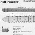 Habakkuk: how the British tried to build an aircraft carrier from ice Why the project was curtailed